1 Particle Sources and Beam Distributions
Discussion Topics…
- \(e\)-, \(p\)+, HI; \(p\)-, \(e\)+, \(\pi\), \(K\), \(\mu\), \(\nu\) beam production
- phase space (transverse, longitudinal), emittance, Liouville
- adiabaticity and its role – normalized emittance
- moments and their transformation; ellipse coefficients
- statistical processes and the Central Limit Theorem
Homework Problem 1:
Npar = 1000Take a random distribution of 1000 particles in (\(x,x'\)), obeying a Gaussian distribution with standard deviations of \(\sigma_x\) = 1 mm and \(\sigma_{x'}\) = 1 milliradian (mr).
- create a scatter plot of \(x'\) vs. \(x\)
- create histograms of the \(x\) and \(x'\) distributions
- extra: create a plot of intensity (density) in the \(x\)-\(x'\) plane
x  = rnorm(Npar,0,1)
xp = rnorm(Npar,0,1)
plot(x,xp)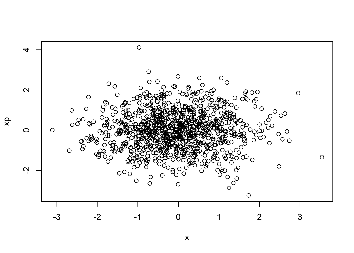
hist(x)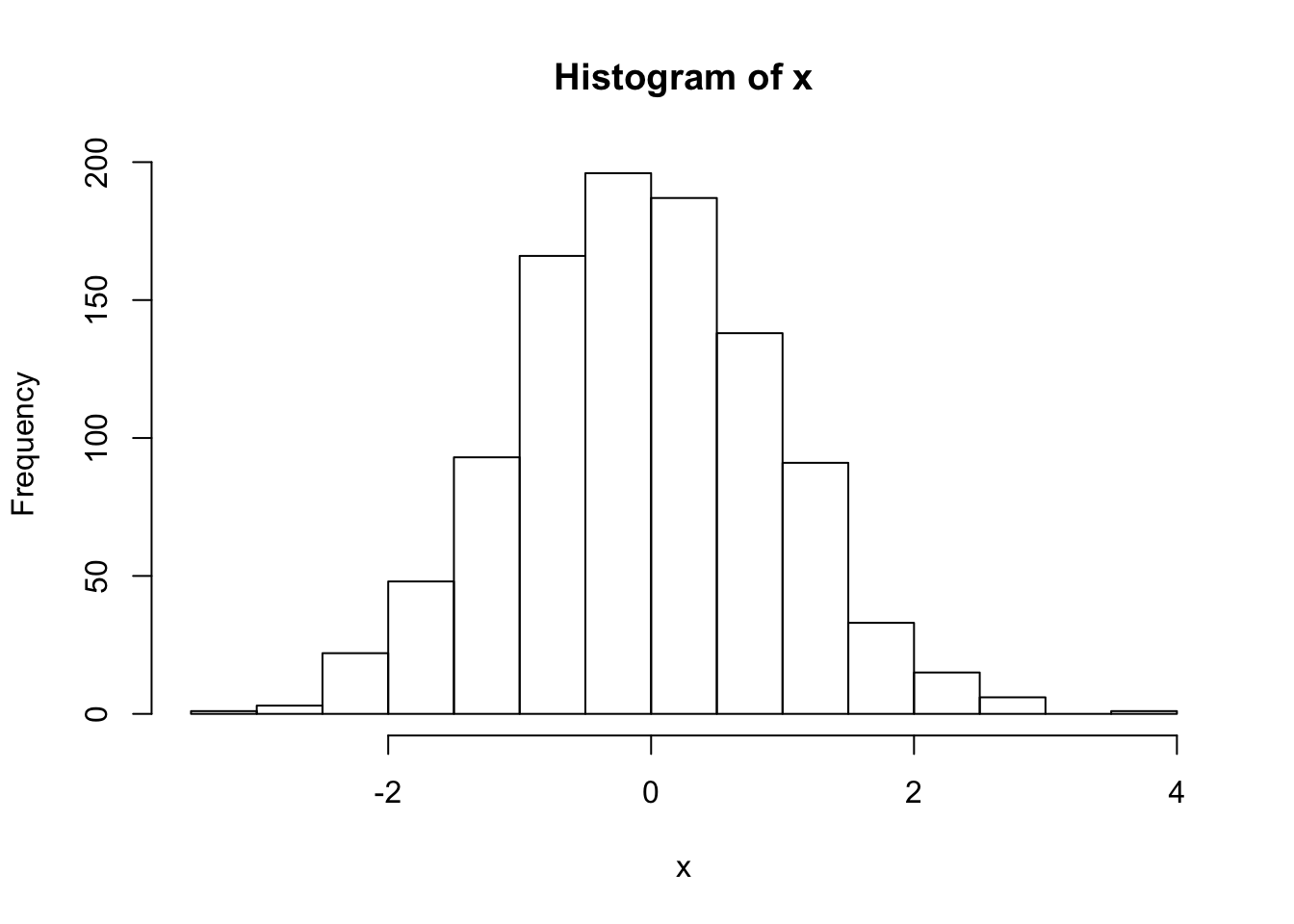
hist(xp)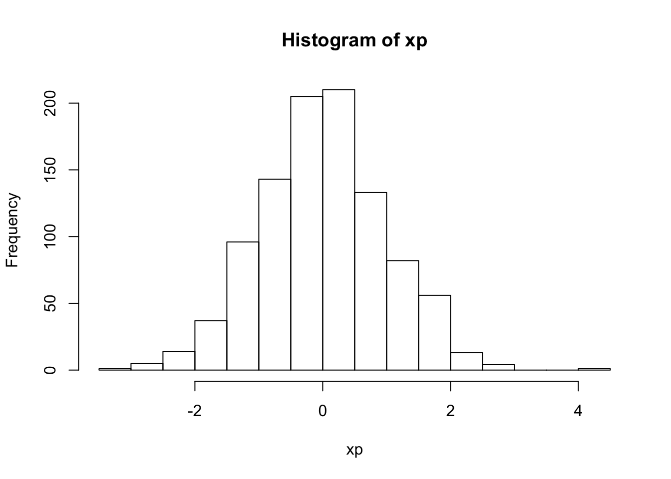
# Other options, just for fun...
df <- data.frame(x,xp)
d <- ggplot(df)
d + geom_bin2d(aes(x,xp),bins=30)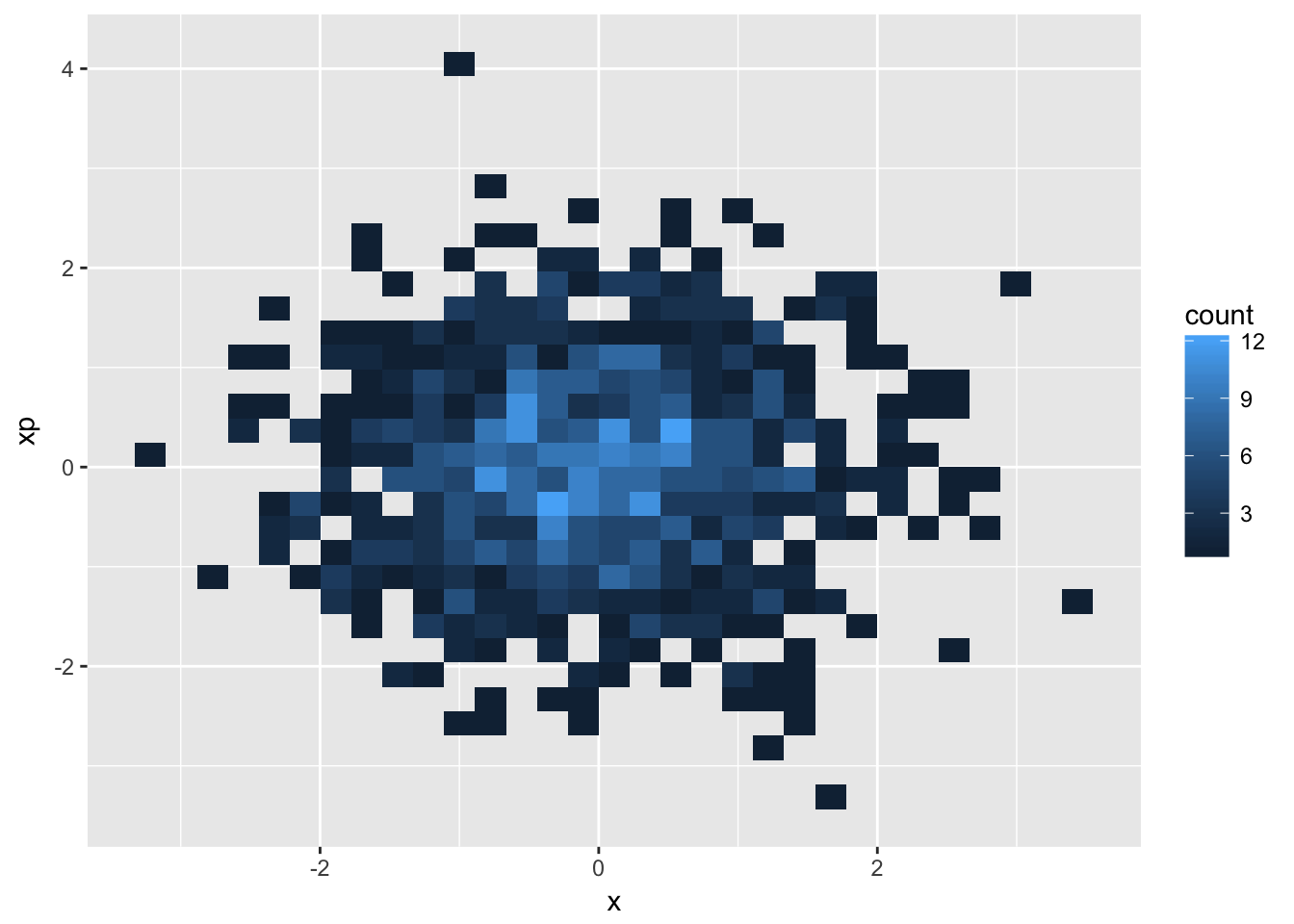
d + geom_density_2d(aes(x,xp),bins=30)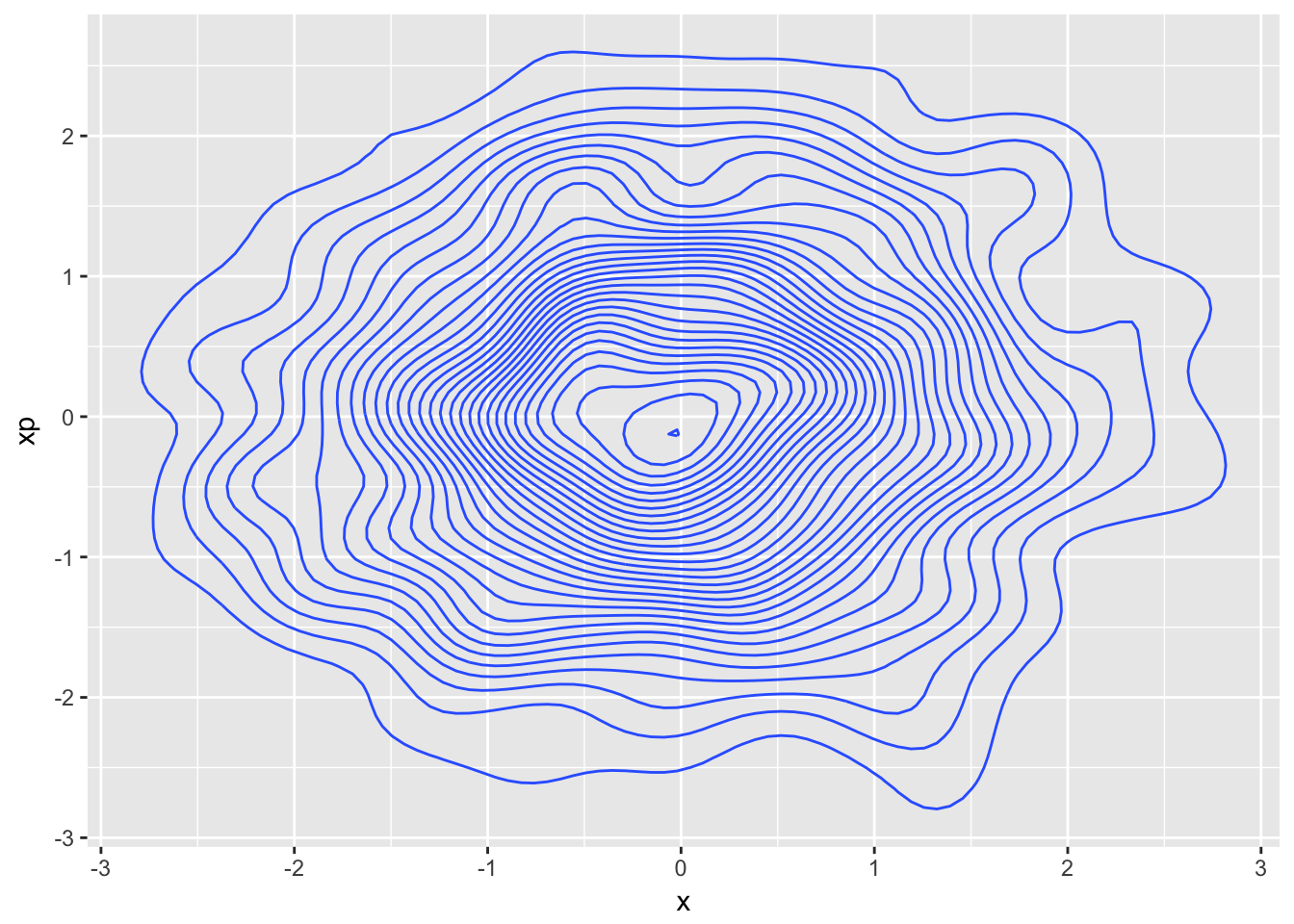
require(KernSmooth)
z <- bkde2D(df, .5)
persp(z$fhat,xlab="x",ylab="xp",theta=30)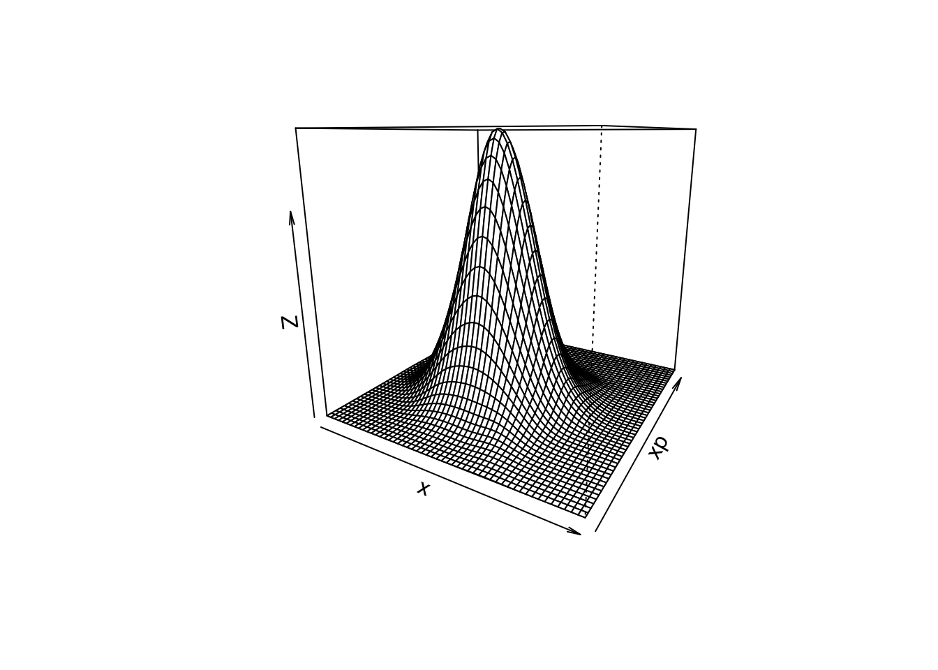
- Allow the particles to drift a distance of \(L\) = 5 m; determine the resulting distributions and compare with those found above
L = 5
xnew = x + L*xp
xpnew = xp
plot(xnew,xpnew)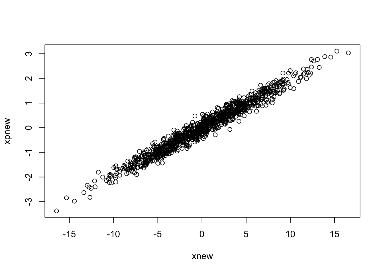
hist(xnew)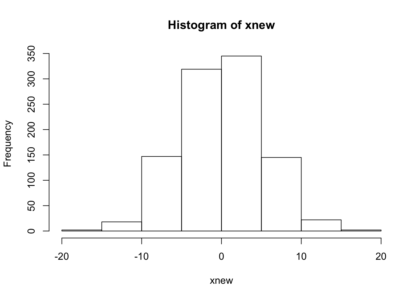
hist(xpnew)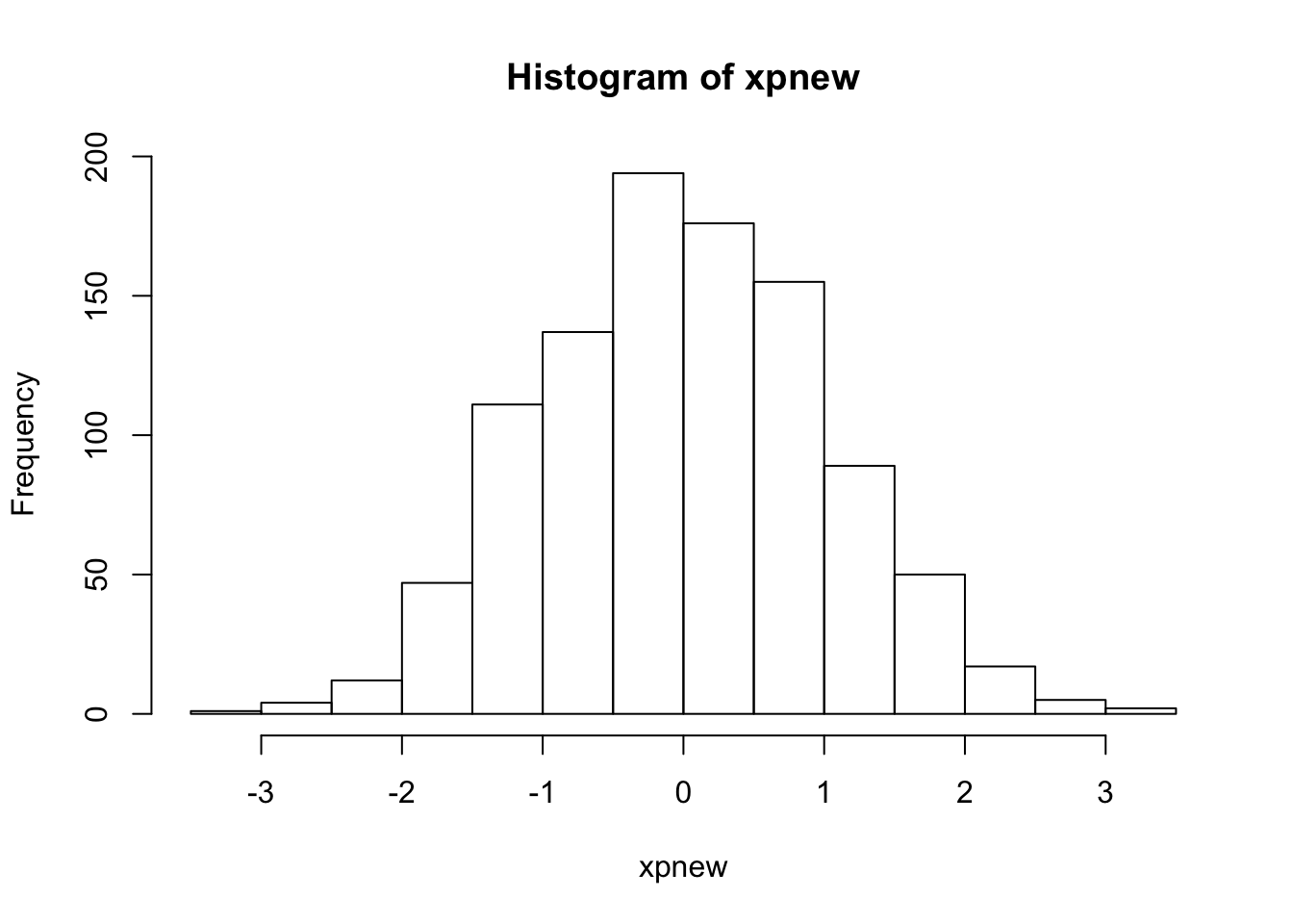
sig2x = var(xnew)
fcn.1 = function(x) Npar*exp(-x^2/2/sig2x)/sqrt(2*pi*sig2x)
hist(xnew)
curve(fcn.1,-5*sqrt(sig2x),5*sqrt(sig2x),add=TRUE)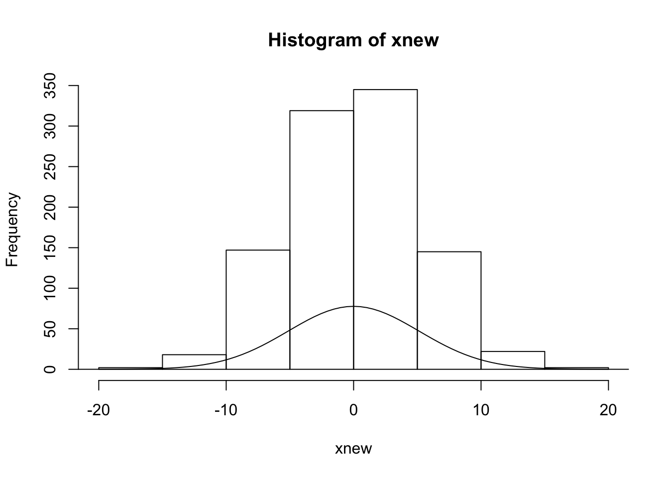
- how should \(x_{rms}\) vary with \(L\)? \((x')_{rms}\) with \(L\)?
- compare the numerical results with the predictions and discuss
- compute the statistical emittance both before and after the drift and compare
- note: \(\epsilon = \sqrt{var(x)var(x')-cov(x,x')^2}\)
# Look at some statistics:
sqrt(var(x))     # rms beam size, mm
[1] 1.002184
sqrt(var(xp)) # rms angular spread, mr[1] 1.014792
bmsize <- function(x) sqrt(1+x^2)
curve(bmsize,0,5,ylim=c(0,6))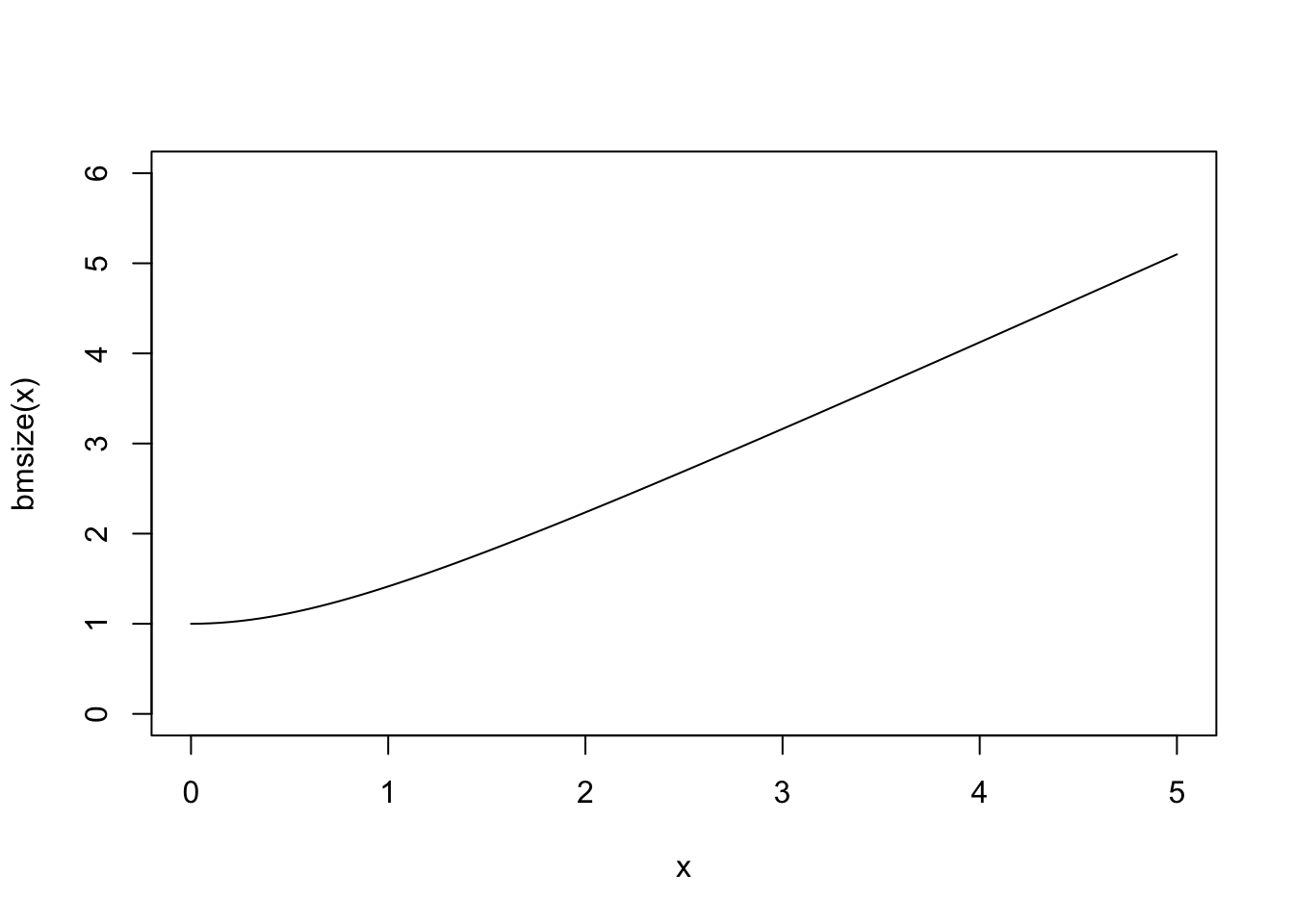
sqrt(var(xnew)) # new rms beam size, mm[1] 5.137072
sqrt(var(x)+L^2*var(xp)) # expected new rms beam size, mm[1] 5.171986
sqrt(var(x)*var(xp)-cov(x,xp)^2) # initial emittance, mm-mr[1] 1.016372
sqrt(var(xnew)*var(xpnew)-cov(xnew,xpnew)^2) # final emittance, mm-mr[1] 1.016372
- From the above results, confirm that \(\Sigma_2 = M \Sigma_1 M^T\), where \[ \Sigma = \left( \begin{array}{cc} var(x) & cov(x,x') \\ cov(x,x') & var(x') \end{array}\right) \] \[ M = \left( \begin{array}{cc} 1 & L \\ 0 & 1 \end{array}\right) \] Note: \(var(x) \equiv \langle x^2 \rangle\), \(cov(x,y) = \langle xy \rangle\).
Sig0 = matrix(c(var(x), cov(x,xp),
             cov(x,xp), var(xp)), nrow=2, byrow=TRUE)

M  = matrix(c( 1, L,
               0, 1 ), nrow=2,byrow=TRUE)
Sig1  = M %*% Sig0 %*% t(M)

Sig1track = matrix(c( var(xnew),       cov(xnew,xpnew),
                      cov(xnew,xpnew), var(xpnew)),
   nrow=2,byrow=TRUE)

# print out results...
Sig0
## [,1] [,2]
## [1,] 1.005166059 0.004859711
## [2,] 0.004859711 0.985959891Sig1## [,1] [,2]
## [1,] 25.702760 4.9346592
## [2,] 4.934659 0.9859599Sig1track## [,1] [,2]
## [1,] 26.389511 5.113021
## [2,] 5.113021 1.029803Homework Problem 2:
set.seed(34)  # set seed
thet = runif(1)*pi/2  # create a value for theta of our rotation matrix
Nstp = 1000   # input set of final rotations to perform
dy = 0.05     # value of random "error" used during tracking
For illustrative purposes, consider a dynamical system wherein the coordinate \(x\) represents transverse position and the coordinate \(y\) represents transverse angles or velocities. A particle undergoes simple harmonic motion in this system, whereby it obeys circular motion in phase space during a “time step”, according to \[ \left( \begin{array}{c} x \\ y \end{array} \right)_{n+1} = \left( \begin{array}{cc} ~~\cos\theta & \sin\theta \\ -\sin\theta & \cos\theta \end{array} \right) \left( \begin{array}{c} x \\ y \end{array} \right)_{n{}} . \] For our exercise, let \(\theta\) = 40 degrees.
Suppose we have an ensemble of 1000 particles and suppose that the initial particle distribution is cylindrically symmetric in phase space according to a bi-Gaussian distribution with \(\sigma_x\) = \(\sigma_y\) = 1. Next, imagine that after each “time step” rotation in phase space by angle \(\theta\), a small random “error” in the \(y\) coordinate, \(\Delta y\), is introduced to each individual particle. (Each particle receives its own, independent error.) The error in \(y\) that is introduced is itself taken from a Gaussian distribution with \(\sigma\) = 0.05.
Create a numerical model of this situation and plot the resulting distribution in phase space after a total number of time steps \(N_s\) = 1000. Determine the resulting rms beam size (\(\langle x^2 \rangle^{1/2}\)) at the end of the time steps. Comment on the shape of the resulting distribution in phase space.
Repeat the above exercise, this time using an initial distribution in phase space that is uniformly distributed within a circle of total extent \(r = x_{max} = y_{max}\) = 1.
Repeat the above two exercises for both (a) Gaussian and (b) uniform initial distributions in phase space, but rather than have our random “errors” picked from a Gaussian distribution, have them picked randomly between three possible values: \(\Delta y\) = {-0.05, 0.00, 0.05}. What can you say about the general form of the resulting distributions?
# We will use Npar particles, and track through Nstp time steps
Npar
## [1] 1000Nstp## [1] 1000# for our value of theta,
thet*180/pi## [1] 40.02917# define the rotation matrix for our particle tracking:
Rmat = matrix(c( cos(thet), sin(thet),
-sin(thet), cos(thet)), ncol=2,byrow=TRUE)
Rmat## [,1] [,2]
## [1,] 0.7657171 0.6431775
## [2,] -0.6431775 0.7657171# For (1-a) Gaussian initial distribution, with Gaussian random errors
#
# set up an array for tracking particles
V <- array(0, dim=c(Npar,Nstp,2))
# set the initial x-y coordinates
V[,1,] = c(rnorm(Npar,0,1),rnorm(Npar,0,1))
plot(V[,1,], xlim=c(-5,5),ylim=c(-5,5), asp=1, pch=".",
xlab="x0", ylab="y0")
hist(V[,1,1], main="x distribution", xlab="x",breaks=20,xlim=c(-6,6))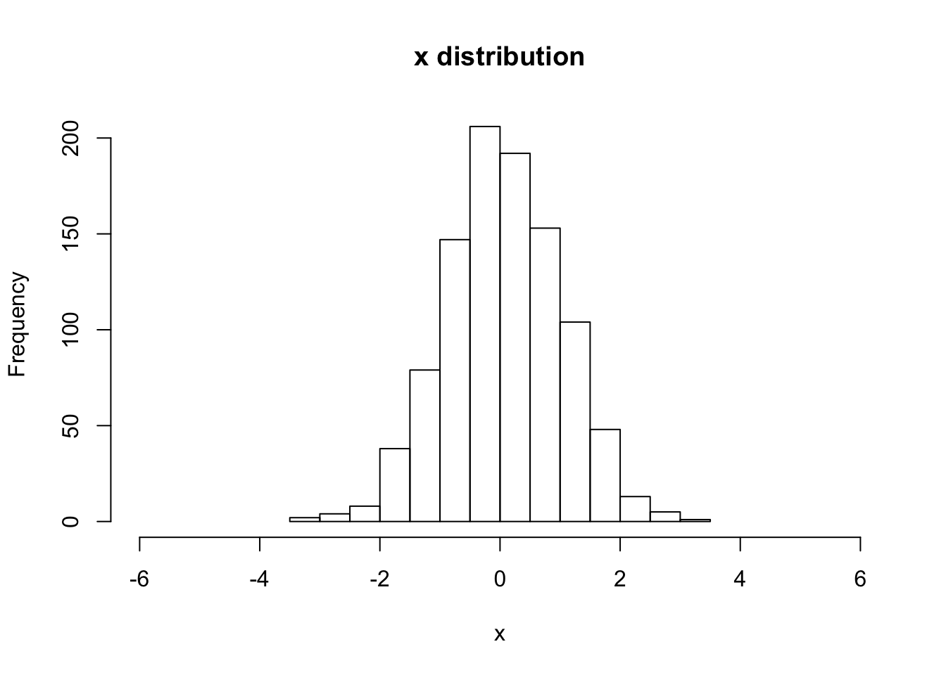
# print the rms x value
sqrt(var(V[,1,1]))
## [1] 0.9651805# begin to loop over the number of steps
j=1
while(j<Npar){
i=1
while(i<Nstp){
vdely = c(0,rnorm(1,0,dy))
V[j,i+1,] = Rmat %*% V[j,i,] + vdely
i = i+1
}
j = j+1
}
plot(V[,Nstp,], xlim=c(-5,5),ylim=c(-5,5), asp=1, pch=".",
xlab="xN", ylab="yN")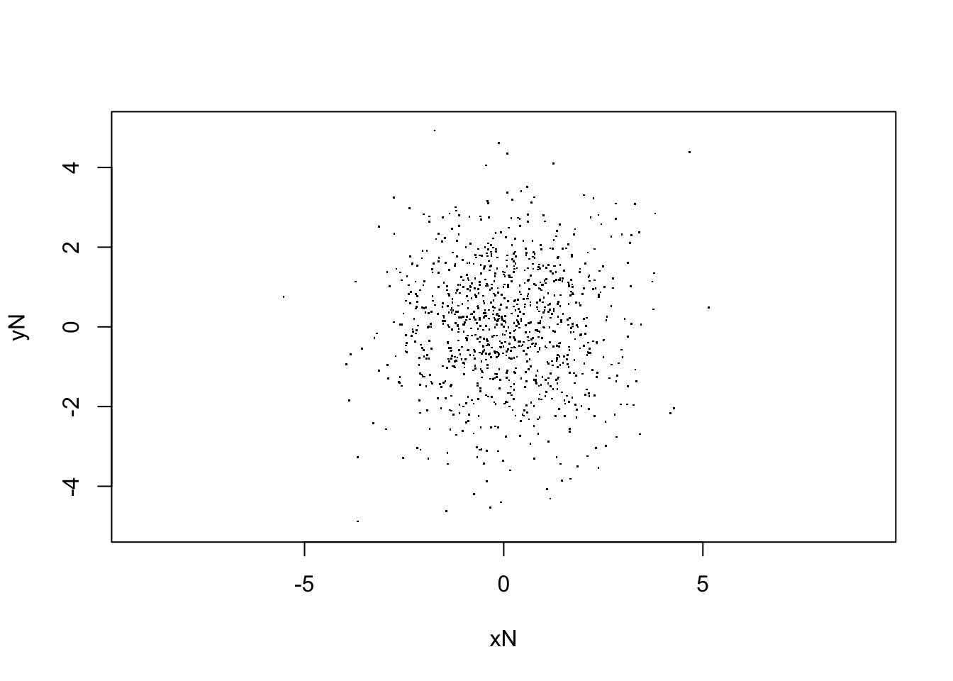
hist(V[,Nstp,1], main="x distribution", xlab="x",breaks=20,xlim=c(-6,6))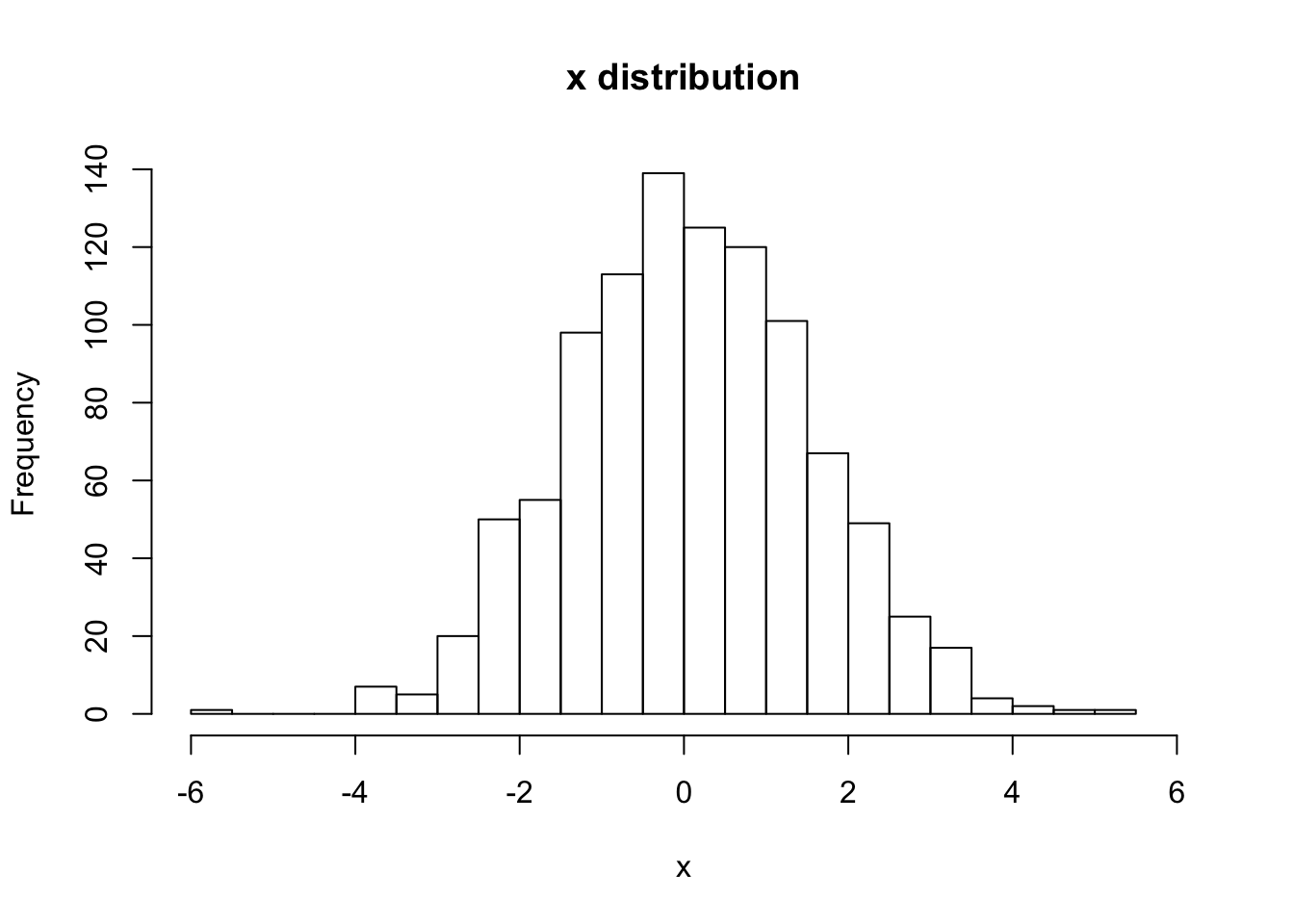
# print out the final rms x-value
sqrt(var(V[,Nstp,1]))
## [1] 1.466122# For (1-b) Uniform initial distribution, with Gaussian random errors
#
# set up an array for tracking particles
V <- array(0, dim=c(Npar,Nstp,2))
# set the initial x-y coordinates
r0 = sqrt(runif(Npar,0,1))
ang = runif(Npar,0,2*pi)
V[,1,] = r0*c(cos(ang),sin(ang))
plot(V[,1,], xlim=c(-5,5),ylim=c(-5,5), asp=1, pch=".",
xlab="x0", ylab="y0")
hist(V[,1,1], main="x distribution", xlab="x",breaks=20,xlim=c(-6,6))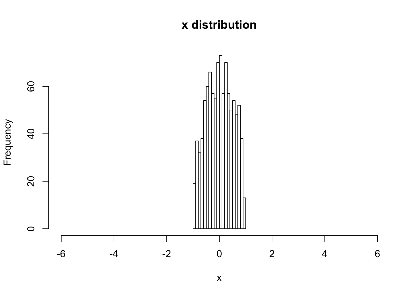
# print the rms x value
sqrt(var(V[,1,1]))
## [1] 0.4983348# begin to loop over the number of steps
j=1
while(j<Npar){
i=1
while(i<Nstp){
vdely = c(0,rnorm(1,0,dy))
V[j,i+1,] = Rmat %*% V[j,i,] + vdely
i = i+1
}
j = j+1
}
plot(V[,Nstp,], xlim=c(-5,5),ylim=c(-5,5), asp=1, pch=".",
xlab="xN", ylab="yN")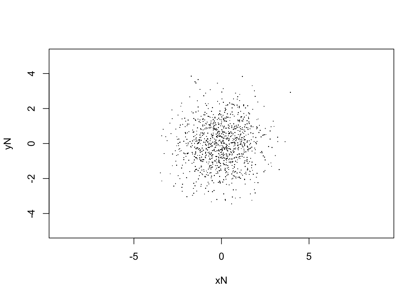
hist(V[,Nstp,1], main="x distribution", xlab="x",breaks=20,xlim=c(-6,6))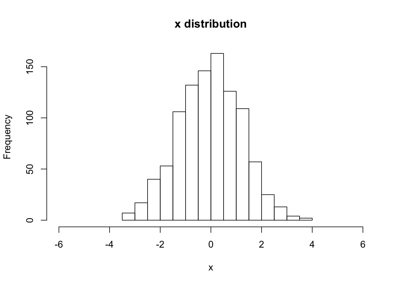
# print out the final rms x-value
sqrt(var(V[,Nstp,1]))
## [1] 1.238252# For (2-a) Gaussian initial distribution, with "pick-3" random errors
#
# set up an array for tracking particles
V <- array(0, dim=c(Npar,Nstp,2))
# set the initial x-y coordinates
V[,1,] = c(rnorm(Npar,0,1),rnorm(Npar,0,1))
plot(V[,1,], xlim=c(-5,5),ylim=c(-5,5), asp=1, pch=".",
xlab="x0", ylab="y0")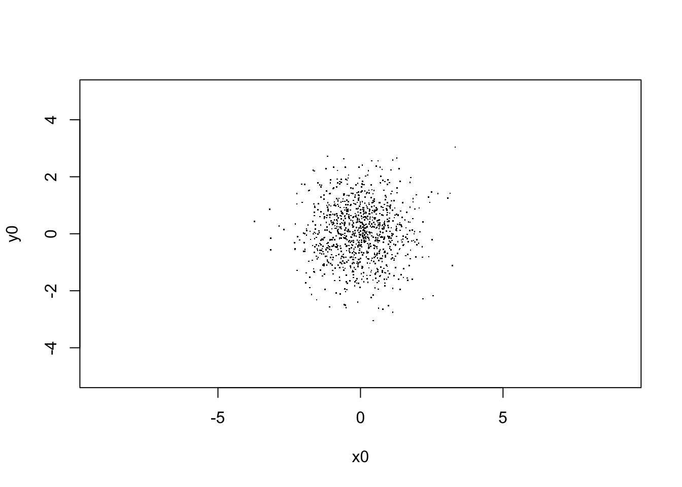
hist(V[,1,1], main="x distribution", xlab="x",breaks=20,xlim=c(-6,6))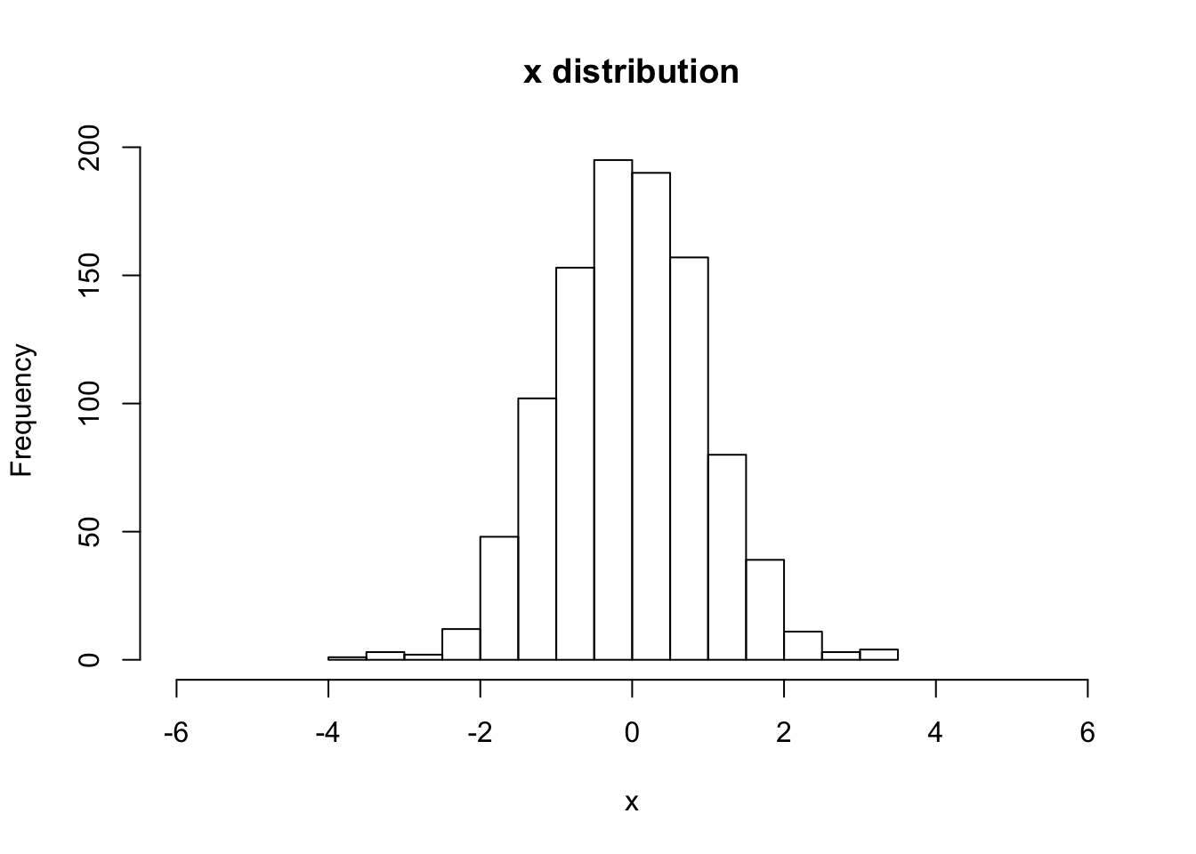
# print the rms x value
sqrt(var(V[,1,1]))
## [1] 0.983273# begin to loop over the number of steps
j=1
while(j<Npar){
i=1
while(i<Nstp){
vdely = c(0,dy*(ceiling(runif(1,0,3))-2))
V[j,i+1,] = Rmat %*% V[j,i,] + vdely
i = i+1
}
j = j+1
}
plot(V[,Nstp,], xlim=c(-5,5),ylim=c(-5,5), asp=1, pch=".",
xlab="xN", ylab="yN")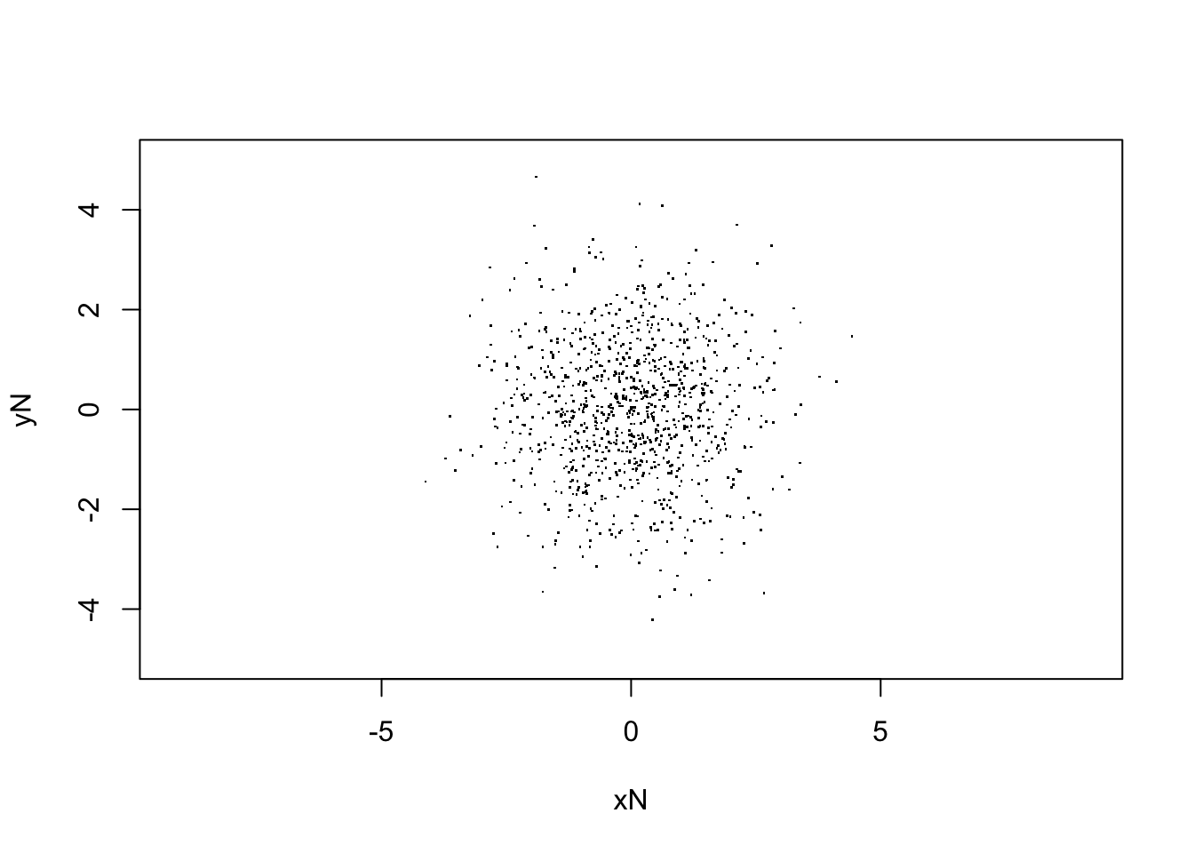
hist(V[,Nstp,1], main="x distribution", xlab="x",breaks=20,xlim=c(-6,6))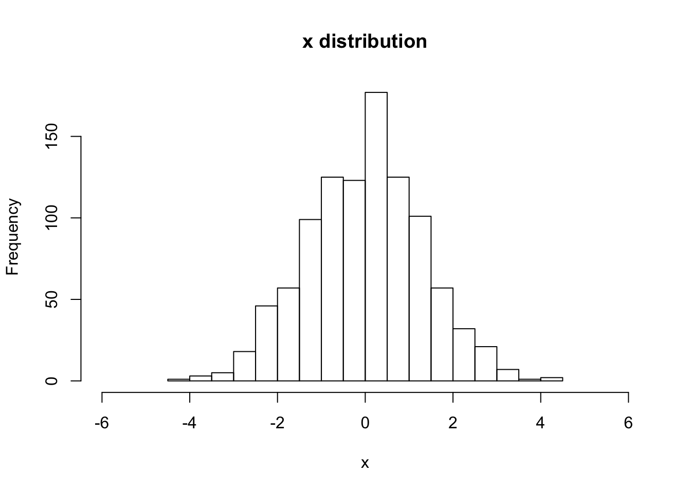
# print out the final rms x-value
sqrt(var(V[,Nstp,1]))
## [1] 1.31636# For (2-b) Uniform initial distribution, with "pick-3" random errors
#
# set up an array for tracking particles
V <- array(0, dim=c(Npar,Nstp,2))
# set the initial x-y coordinates
r0 = sqrt(runif(Npar,0,1))
ang = runif(Npar,0,2*pi)
V[,1,] = r0*c(cos(ang),sin(ang))
plot(V[,1,], xlim=c(-5,5),ylim=c(-5,5), asp=1, pch=".",
xlab="x0", ylab="y0")
hist(V[,1,1], main="x distribution", xlab="x",breaks=20,xlim=c(-6,6))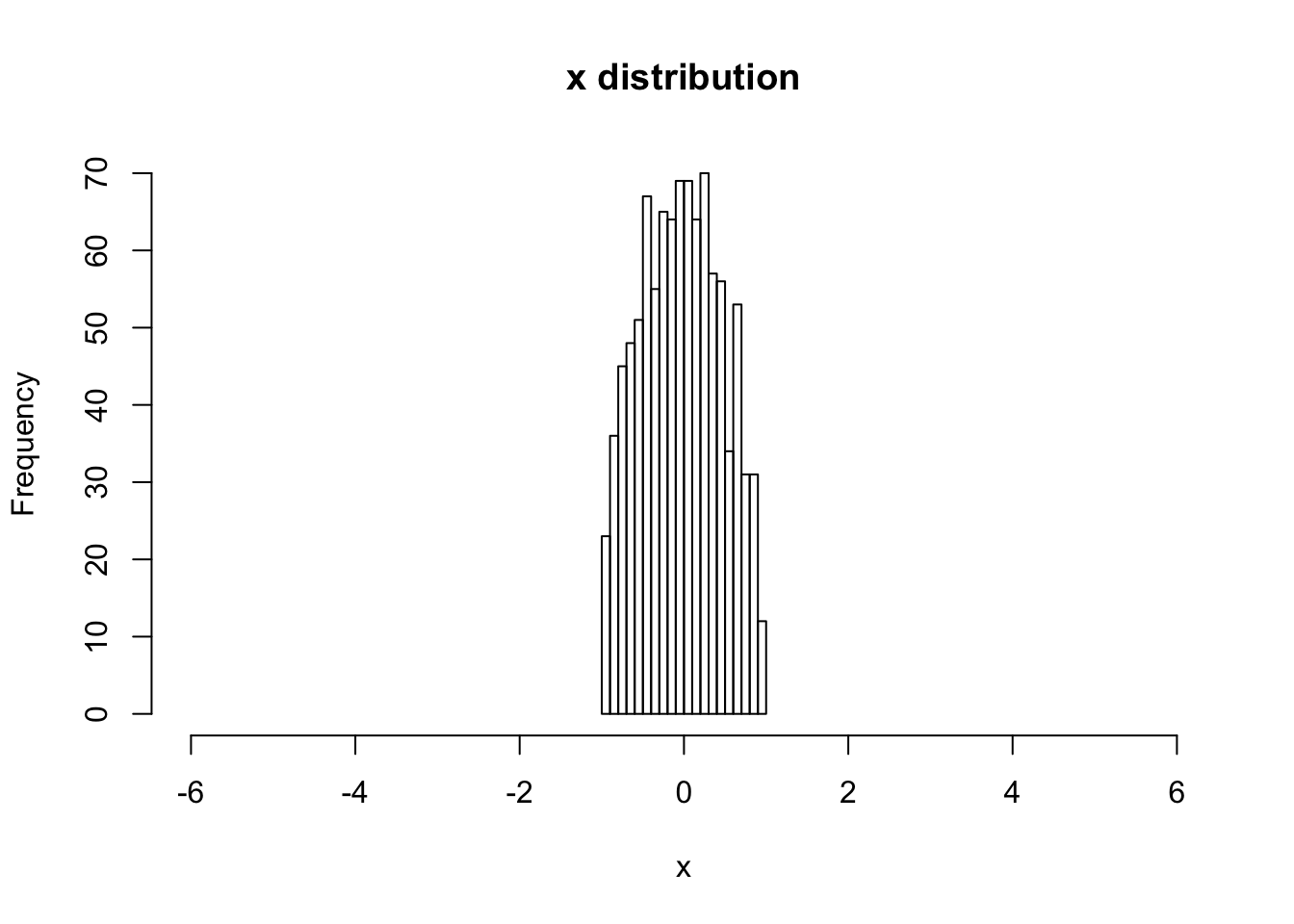
# print the rms x value
sqrt(var(V[,1,1]))
## [1] 0.4905073# begin to loop over the number of steps
j=1
while(j<Npar){
i=1
while(i<Nstp){
vdely = c(0,dy*(ceiling(runif(1,0,3))-2))
V[j,i+1,] = Rmat %*% V[j,i,] + vdely
i = i+1
}
j = j+1
}
plot(V[,Nstp,], xlim=c(-5,5),ylim=c(-5,5), asp=1,
xlab="xN", ylab="yN", pch=".")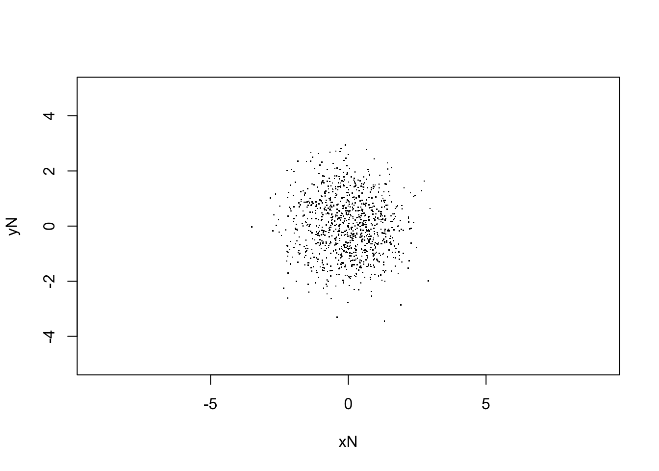
hist(V[,Nstp,1], main="x distribution", xlab="x",breaks=20,xlim=c(-6,6))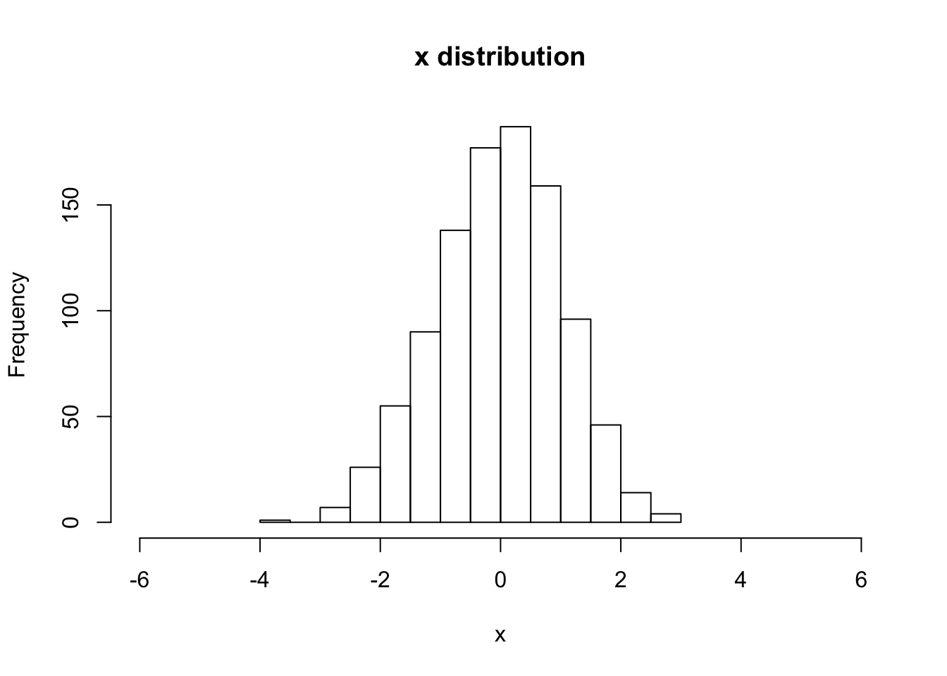
# print out the final rms x-value
sqrt(var(V[,Nstp,1]))
## [1] 1.042113