5 Courant-Snyder Theory of Transverse Motion
Discussion Topics…
- General Equation of Motion (Hill’s Equation)
- Piecewise Solution
- Amplitude Function Description
Computations of Beam Envelope
- Linear Errors
- Dispersion and Momentum Compaction
Chromatic Effects and Corrections
Homework Problem 1:
L  = 30
F  = 25
Mf = matrix(c(  1,  0,
              -1/F, 1), nrow=2, ncol=2, byrow=TRUE)
Md = matrix(c(  1,  0,
               1/F, 1), nrow=2, ncol=2, byrow=TRUE)
Mo = matrix(c(  1,  L,
                0,  1), nrow=2, ncol=2, byrow=TRUE)
Mc = Mf %*% Mo %*% Md %*% Mo

N2cells = 48  # No. of half-cells; = 2x no. of full FODO cells
Consider a FODO cell made up of a drift of length \(L\) = 30 m followed by a defocusing quadrupole of focal length \(-F\) = -25 m followed by a drift of length \(L\) followed by a focusing quadrupole of focal length \(+F\). Using the thin-lens FODO equations, estimate the values of the Courant-Snyder parameters \(\alpha\), \(\beta\), and \(\gamma\) at the exit of the FODO cell.
beta  = array(0,N2cells+1)
alpha = array(0,N2cells+1)
gamma = array(0,N2cells+1)

# Initial values of beta,alpha,gamma:
alpha[1] = sqrt((1+L/2/F)/(1-L/2/F))
beta[1]  = 2*F*alpha[1]
gamma[1] = (1+alpha[1]^2)/beta[1]

alpha[1]
## [1] 2beta[1] # m## [1] 100gamma[1] # 1/m## [1] 0.05We now wish to transport the CS parameters found above through a series of FODO cells. Create the matrix \(K\) using the numerical results above, and compute the values of the CS parameters at the end of each \(F\) and \(D\) quadrupole through a system of 24 FODO cells by propagating the \(K\) matrix according to \[ K_2 = M K_1 M^T \]
# Compute beta through a series of (drift + quad)'s:
MoF = Mf %*% Mo
MoD = Md %*% Mo

K = array(0,dim=c(2,2,N2cells+1))
K[,,1] = matrix(c(beta[1], -alpha[1],
                -alpha[1],  gamma[1]),nrow=2,ncol=2,byrow=TRUE)
K[,,1]
## [,1] [,2]
## [1,] 100 -2.00
## [2,] -2 0.05i = 2
while(i<(N2cells+1)){
K[,,i] = MoD %*% K[,,i-1] %*% t(MoD)
K[,,i+1] = MoF %*% K[,,i] %*% t(MoF)
i = i+2
}
i = 2
while(i<(N2cells+1)){
beta[i] = K[1,1,i]
alpha[i] = -K[1,2,i]
gamma[i] = K[2,2,i]
i = i+1
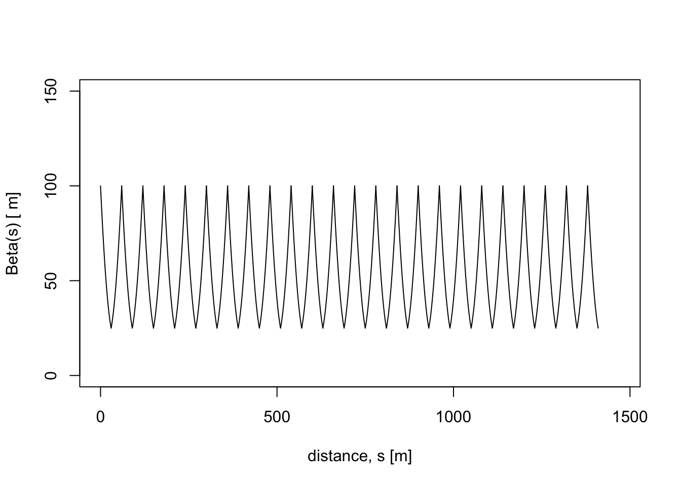
}Plot the results as a function of distance along the FODO system, including the functional form of the amplitude function (\(\beta\)) between the quadrupoles.
# Path length along the FODO system:
s = array(0,N2cells+1)
i=2
while(i<N2cells+2){
   s[i] = s[i-1] + L
   i = i+1
}

# Write a Function to plot beta
bet_0 = beta[1]; alph_0 = alpha[1]
bet <- function(x){
   bet_0 - 2*alph_0*x + (1+alph_0^2)/bet_0*x^2
}

i = 2
plot(0,0,xlim=c(0,L*length(s)), ylim=c(0,1.5*max(beta)),typ="n",
   xlab="distance, s [m]", ylab="Beta(s) [ m]")
while(i<(N2cells+1)){
   alph_0 = alpha[i-1]; bet_0 = beta[i-1]
   curve(bet(x-s[i-1]), s[i-1], s[i], add=TRUE)
   i = i+1
}
Homework Problem 2:
# Create a particle distribution
Npar   <- 100  # number of particles in our distribution
rms0 = 1.0   # mm
Create a collection of 100 particles which has a Gaussian distribution in \(x\) with rms width 1 mm, and which has a phase space distribution consistent with the initial set of Courant-Snyder parameters found in the previous problem. Plot the phase space distribution and histograms of the \(x\) and \(x'\) variables.
# x, xp (= x') will be 2-D arrays
#  1st parameter = particle number
#  2nd parameter = value of x or x'

x   <- array(0, dim=c(Npar,length(s)+1))
p   <- array(0, dim=c(Npar,length(s)+1))
xp  <- array(0, dim=c(Npar,length(s)+1))

x[,1]  <- rnorm(Npar,0,rms0)
p[,1]  <- rnorm(Npar,0,rms0)

# Use pre-given values of beta, alpha
b0 = beta[1]
a0 = alpha[1]
xp[,1] = (p[,1]-a0*x[,1])/b0  # mrad

plot(x[,1],xp[,1],
   xlim=c(-1,1)*max(abs(x)), ylim=c(-1,1)*max(abs(xp)),
   xlab="position x (mm)", ylab="angle x' (mrad)")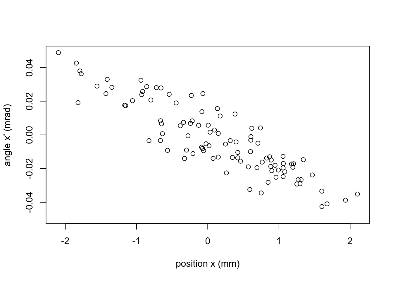
hist(x[,1])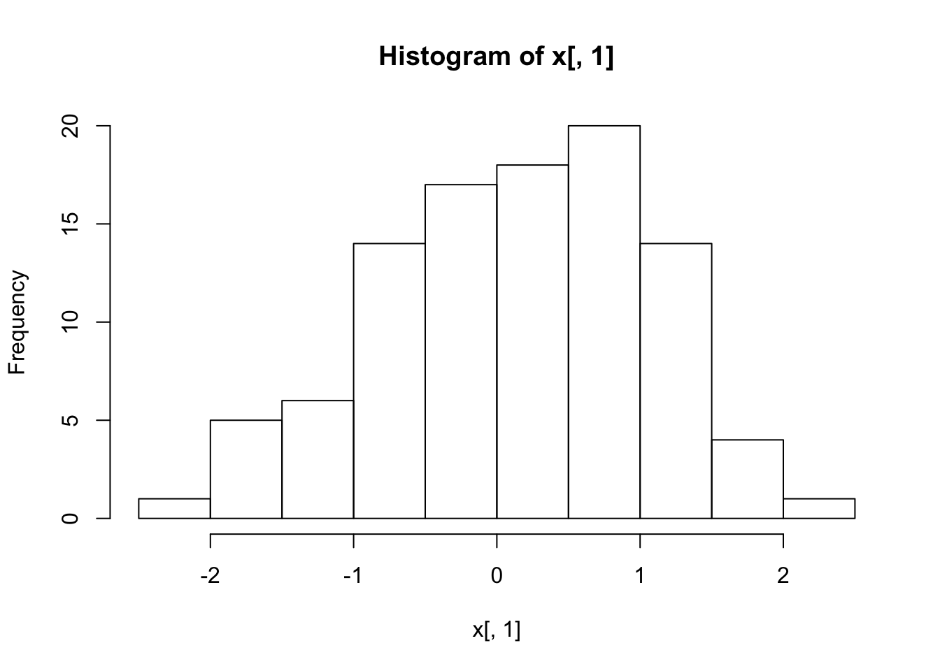
hist(xp[,1])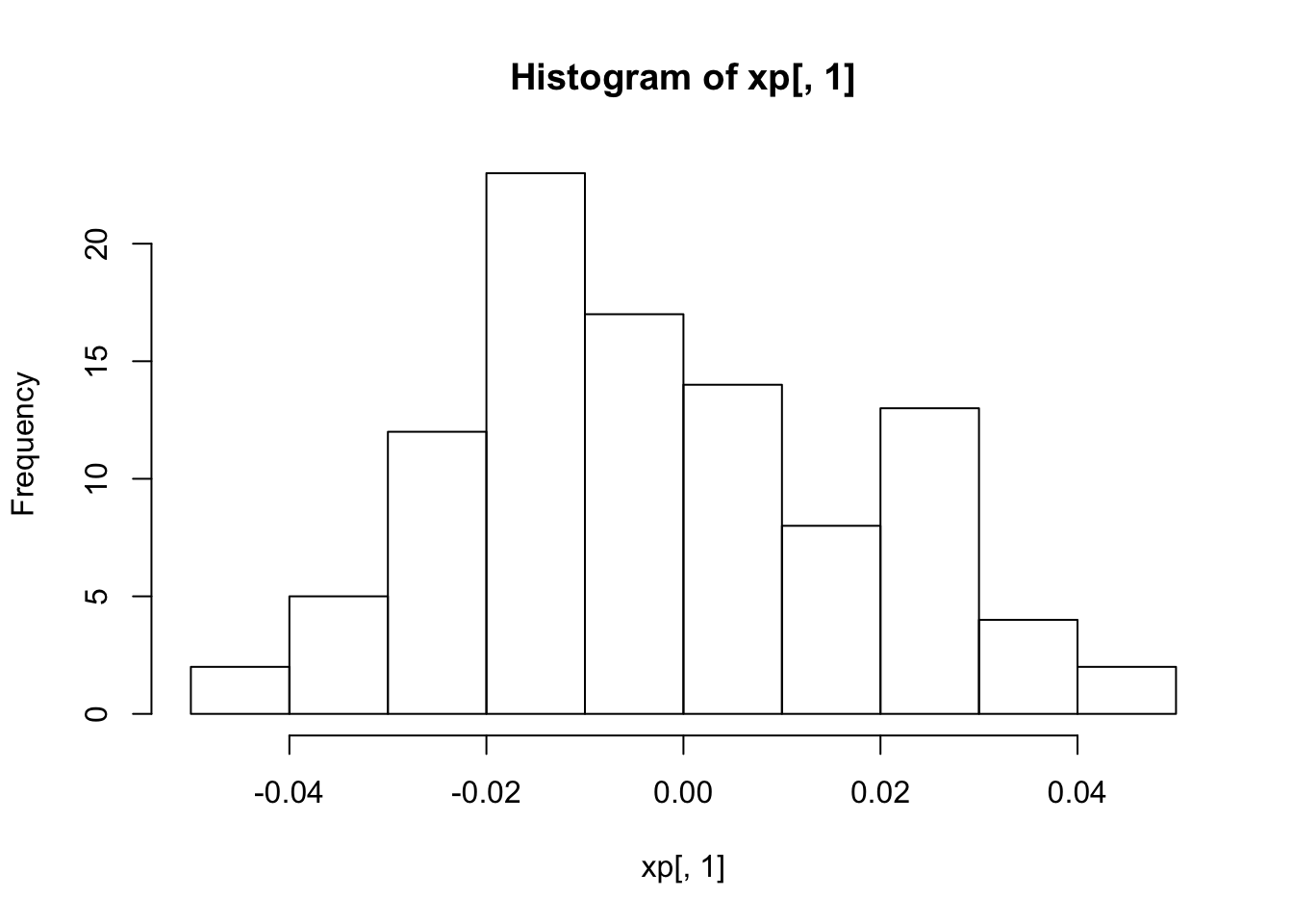
For each particle in the distribution just found, track its phase space coordinates through the system of 24 FODO cells used previously. Trace the trajectory of each particle through the system by plotting its \(x\) coordinate as a function of \(s\). Compare the resulting “envelope” of the trajectories with the function \(\sqrt{\beta}(s)\) (scaled arbitrarily) found in the previous problem.
# Track the distribution through the beam line

plot(0,0,xlim=c(0,L*length(s)),
   ylim=c(-1,1)*1.8*max(abs(x)),typ="n",
   xlab="distance s (m)", ylab="position x (mm)")
q = 1/F
i = 2  # position along the beam line
while(i<(length(s)+1)){
   j = 1
   while(j<(Npar+1)){
      x[j,i]  =  x[j,i-1]  + L*xp[j,i-1]
      xp[j,i] = xp[j,i-1]  -    x[j,i]*q*(-1)^(i+1)
      lines(c(s[i-1],s[i]),c(x[j,i-1],x[j,i]))
      j = j+1
      }
   i = i+1
}
# Add plot of sqrt(beta(s)) to the tracking result
#  scale by arbitrary amount, A
AbsX = abs(x)
imax = which(AbsX == max(AbsX), arr.ind = TRUE)[2]
A = max(abs(x[,imax]))/sqrt(beta[imax])
i = 2
while(i<(length(s)+1)){
   alph_0 = alpha[i-1]; bet_0 = beta[i-1]
   curve( A*sqrt(bet(x-s[i-1])), s[i-1], s[i], add=TRUE, col="blue",lwd=3)
   curve(-A*sqrt(bet(x-s[i-1])), s[i-1], s[i], add=TRUE, col="blue",lwd=3)
   i = i+1
}
text(400,-1.25*max(abs(x)),"blue = ~sqrt(beta(s))")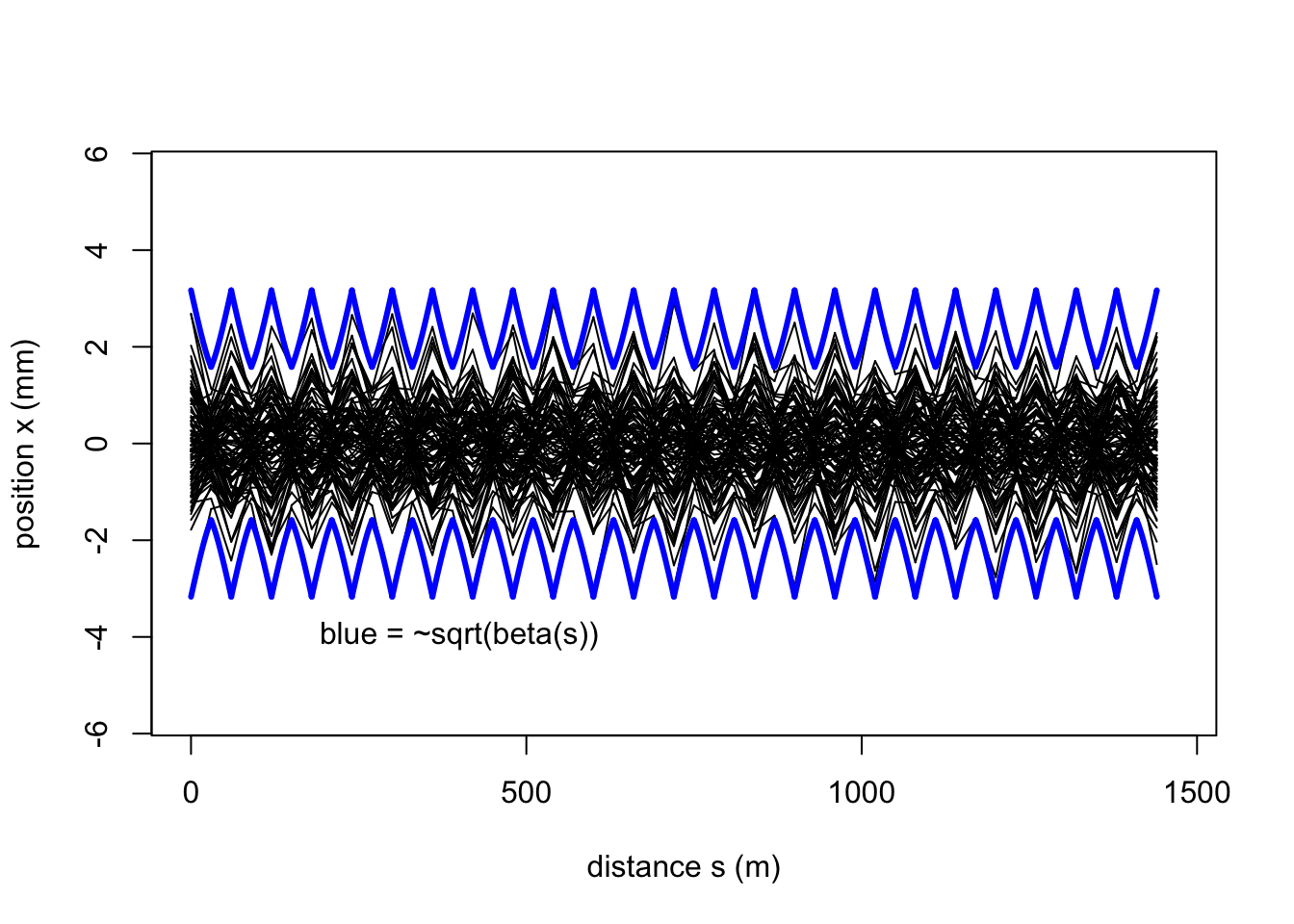
Homework Problem 3:
Nc = 52
thet = 0.01
ierr = 17
xinit = 0.5 # mm
Nrev = 20
Continuing to use our FODO cells from previous problems, consider a closed system of 52 such FODO cells creating a circular accelerator. (We imagine that the O’s in the system are actually bending magnets, but let’s neglect any focusing effects from these.) Imagine that at the end of the 17-th FODO cell (thus, at a “focusing” magnet) a steering error is present that produces an angular deflection of magnitude \(\theta\) = 0.01 each time it is encountered.
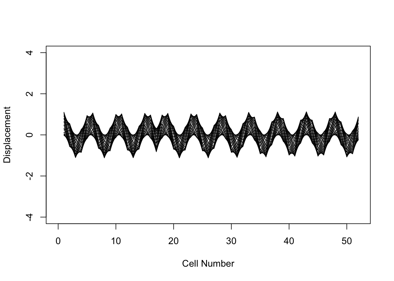
- A particle begins circulating the accelerator at \(s\) = 0 with initial conditions \(x_0\) = 0.5 mm and \(x'_0\) = 0. Plot the trajectory of the particle through the system – including the effect of the steering error – for up to 20 revolutions.
plot(0,0, xlim=c(0,Nc), ylim=c(-1,1)*4, xlab="Cell Number", ylab="Displacement",typ="n")
n = 1    # turn number
X = c(xinit, 0)          # initial particle state vector (x,xp)
xt = array(0,dim=Nc)     # position at end of each cell
while(n<Nrev+1){
  i = 1
  while ( i<(Nc+1) ){
    V = Mc %*% X + ifelse(i == ierr, 1, 0 )*c(0,thet)
    X = V
    xt[i] = X[1]
    i = i+1
  }
  points(c(1:Nc), xt, typ="l")
  n = n+1
}
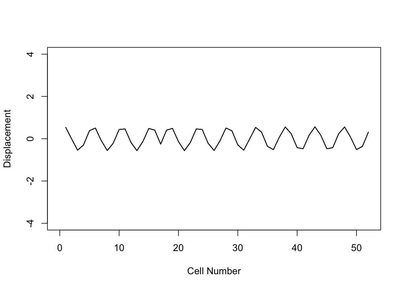
- Next, determine the initial conditions (\(x_0\), \(x'_0\)) at \(s\) = 0 for the closed orbit. Verify your result by tracking this initial condition through the system for 20 revolutions.
 PwrM = function(M,n){     # function to take matrix M to n-th power
   Mout = diag(1,2)
   i = 0
   while (i<n){
     Mout = M %*% Mout
     i = i+1
   }
   Mout
 }

dX = c(0,thet)
 X0 = solve( diag(1,2) - PwrM(Mc,Nc) ) %*% PwrM(Mc,Nc-ierr) %*% dX
X0
## [,1]
## [1,] 0.311670260
## [2,] -0.001552705plot(0,0, xlim=c(0,Nc), ylim=c(-1,1)*4,
xlab="Cell Number", ylab="Displacement",typ="n")
n = 1 # turn number
X = X0 # initial particle state vector (x,xp)
xt = array(0,dim=Nc) # position at end of each cell
while(n<Nrev+1){
i = 1
while ( i<(Nc+1) ){
V = Mc %*% X + ifelse(i == ierr, 1, 0 )*c(0,thet)
X = V
xt[i] = X[1]
i = i+1
}
points(c(1:Nc), xt, typ="l")
n = n+1
}
# Here, we combine the two results into a single plot:

plot(0,0, xlim=c(0,Nc), ylim=c(-1,1)*4,
   xlab="Cell Number", ylab="Displacement",typ="n")
n = 1    # turn number
X = c(xinit, 0)          # initial particle state vector (x,xp)
xt = array(0,dim=Nc)     # position at end of each cell
while(n<Nrev+1){
  i = 1
  while ( i<(Nc+1) ){
    V = Mc %*% X + ifelse(i == ierr, 1, 0 )*c(0,thet)
    X = V
    xt[i] = X[1]
    i = i+1
  }
  points(c(1:Nc), xt, typ="l")
  n = n+1
}
X = X0
xt = array(0,dim=Nc)
i = 1
while ( i<(Nc+1) ){
   V = Mc %*% X + ifelse(i == ierr, 1, 0 )*c(0,thet)
   X = V
   xt[i] = X[1]
   i = i+1
}
points(c(1:Nc), xt, typ="l", col="red", lwd=3)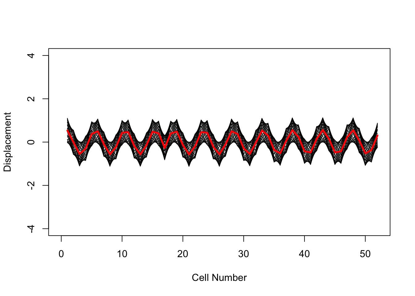
- What is the tune of the FODO accelerator? How do you expect the particle behavior to vary as a function of tune?
# Compute the tune of the system:
mu = acos(sum(diag(Mc))/2)
nu = mu*Nc/2/pi
nu
## [1] 10.6513Homework Problem 4:
Using our system of 52 FODO cells from the previous problem,
- Estimate the horizontal and vertical natural chromaticities of the system. Also, calculate the maximum and minimum values of the dispersion function in the FODO cells, using our thin lens formulas.
xi_est = -nu   # same for each plane, x/y
xi_est
## [1] -10.6513beta_max = 2*F*sqrt( (1+sin(mu/2))/(1-sin(mu/2)) )
beta_min = 2*F*sqrt( (1-sin(mu/2))/(1+sin(mu/2)) )
theta0 = 2*pi/Nc/2 # bending angle per half-cell
D_max = L*theta0/sin(mu)^2*(1 + 1/2*sin(mu/2))
D_min = L*theta0/sin(mu)^2*(1 - 1/2*sin(mu/2))
D_max; D_min # meters## [1] 2.556635## [1] 1.376649- We now wish to adjust the chromaticities of the synchrotron using two sextupole families to generate \(\xi_x = \xi_y\) = 0. Find the “sextupole strengths” \(S_1\) and \(S_2\) required to do this, with \(S_1\) corresponding to sextupoles at the Focusing (\(x\)) quadrupole locations and \(S_2\) corresponding to sextupoles at the Defocusing (\(x\)) quadrupole locations. Note:
\[ S \equiv \frac{\partial^2 B_y/\partial x^2\; \ell}{2B\rho} \]
#  dxi_x =  Nc/2/pi * [ (beta_max*D_max)*S1 + (beta_min*D_min)*S2 ]
#  dxi_y = -Nc/2/pi * [ (beta_min*D_max)*S1 + (beta_max*D_min)*S2 ]
#
#    So, ...
#      our target vector is:
dxi = -xi_est*c(1,1)
#
C = Nc/2/pi * matrix( c( beta_max*D_max,  beta_min*D_min,
                        -beta_min*D_max, -beta_max*D_min),
     nrow=2, byrow=TRUE)
S = solve(C) %*% dxi
S  # 1/m^2
## [,1]
## [1,] 0.00671196
## [2,] -0.01246507# Check:
C %*% S - dxi## [,1]
## [1,] -1.776357e-15
## [2,] 0.000000e+00pc = 30 # GeV
Brho = 10/2.9979*pc # T-m
Rsxt = 0.1 # m
Lsxt = 0.2 # m- If the particle momentum is \(p\) = 30 GeV/c, and if the sextupoles are each 0.2 m long and each have a pole tip radius of 10 cm, what will be the magnetic field strengths required (measured at the sextupole magnet pole tips) to bring the chromaticity to zero in each plane?
dBppL = 2*Brho*S
dBppL  # Tesla/m
## [,1]
## [1,] 1.343332
## [2,] -2.494760dB = dBppL*Rsxt^2/2/Lsxt
dB # Tesla; F-quad and D-quad locations, respectively## [,1]
## [1,] 0.03358331
## [2,] -0.06236900