2 Guiding Particles and Keeping Them Focused
Discussion Topics…
- Electrostatic Devices
- Magnetic Devices
- Rigidity
- Solenoids, and when (not) to use them
- Global vs. Local Coordinates
- Quadrupoles as Lenses
- Doublets, Triplets; FODO System
Homework Problem 1:
theta = 45*pi/180
rho = 0.25 # m
Wmax = 20 # MeV
Suppose we wish to bend a proton’s trajectory by 45 degrees, with a bending radius of 0.25 m, by (a) electrostatic deflection or (b) by magnetic deflection.
For (a) plot the value of the electric field required along a circular (equipotential) trajectory within a cylindrical bend as a function of the proton’s kinetic energy, up to 20 MeV. What path length is required? Neglect edge effects. Note: A practical engineering limit for an electric field in this problem is about \(E_{max} \approx\) 20 MV/m.
#F = eE = gamma m v^2/R = gamma E0 beta^2 / R
#  = gamma beta^2 E0/R = (beta*gamma)^2/gamma E0/R
#  = (gamma^2 - 1)/gamma E0/R  =  (gamma-1)(gamma+1)/gamma E0/R
#  = (W/E0)(W/E0+2)/(1+W/E0) E0/R;  x == W/E0
E0 = 938       # MeV
E = function(x) {x*(2+x)/(1+x)*E0/rho} # MV/mcurve(E(x/E0),0,Wmax,
xlab="kinetic energy (MeV)", ylab="E (MV/m)")
abline(h=20, lty=2)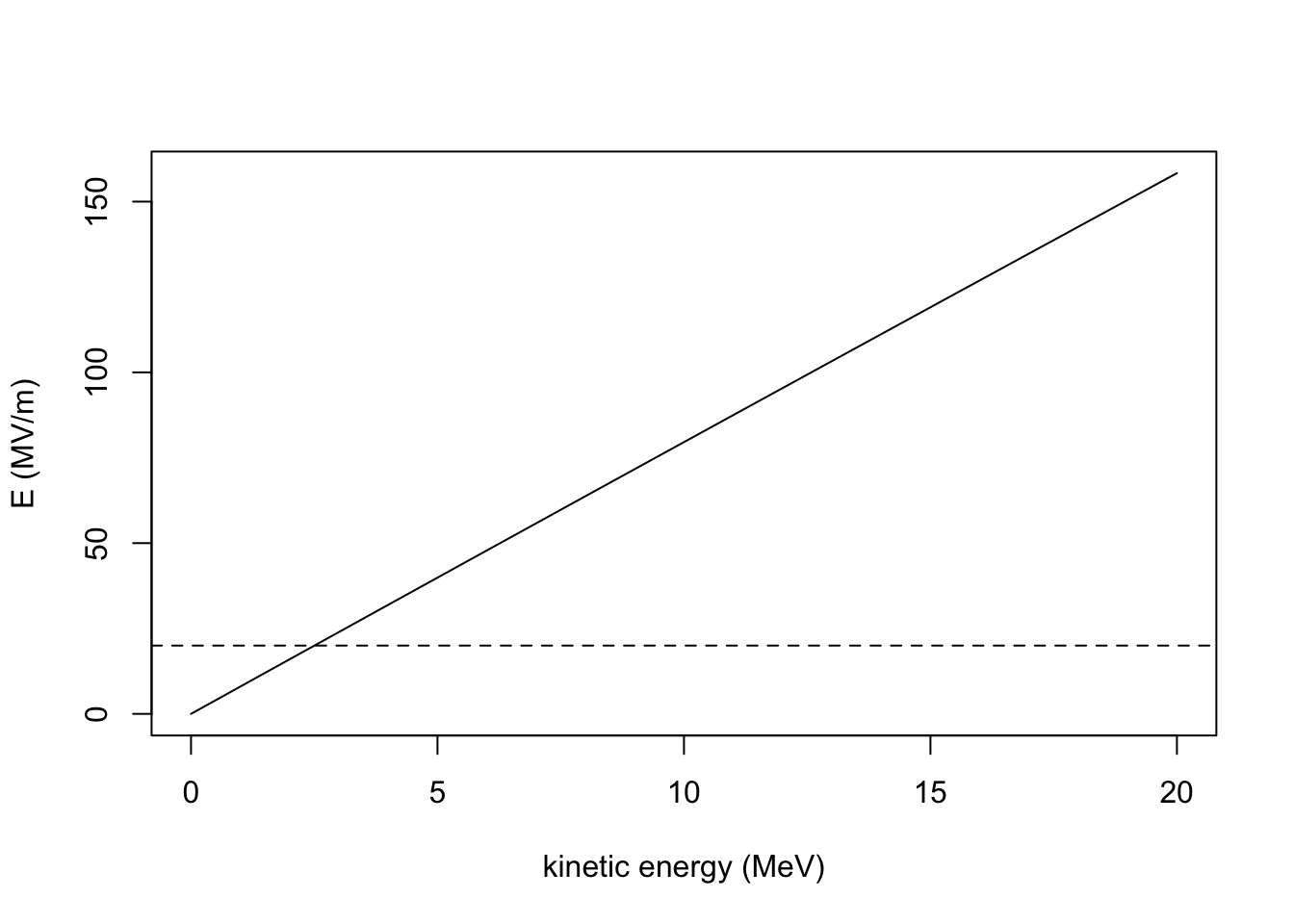
Le = rho*theta
Le # m
## [1] 0.1963495For (b) plot the magnetic field strength required in an electromagnet as a function of the proton’s kinetic energy. Again, neglect edge effects. Note: A practical engineering limit for a magnetic field in this problem is about \(B_{max} \approx\) 2 T.
# Brho = p/e = pc/ec = 10/2.9979*pc[GeV]
# pc = E0 sqrt(gamma^2-1) = E0 sqrt(W/E0 * (2+W/E0))
# B = Brho/rho = 10/2.9979*(E0/1000)/rho * sqrt(W/E0 * (2+W/E0))
B = function(x){ 10/2.9979*(E0/1000)/rho*sqrt(x*(2+x)) } # Teslacurve(B(x/E0),0,Wmax,
xlab="kinetic energy (MeV)", ylab="B (T)")
abline(h=2, lty=2)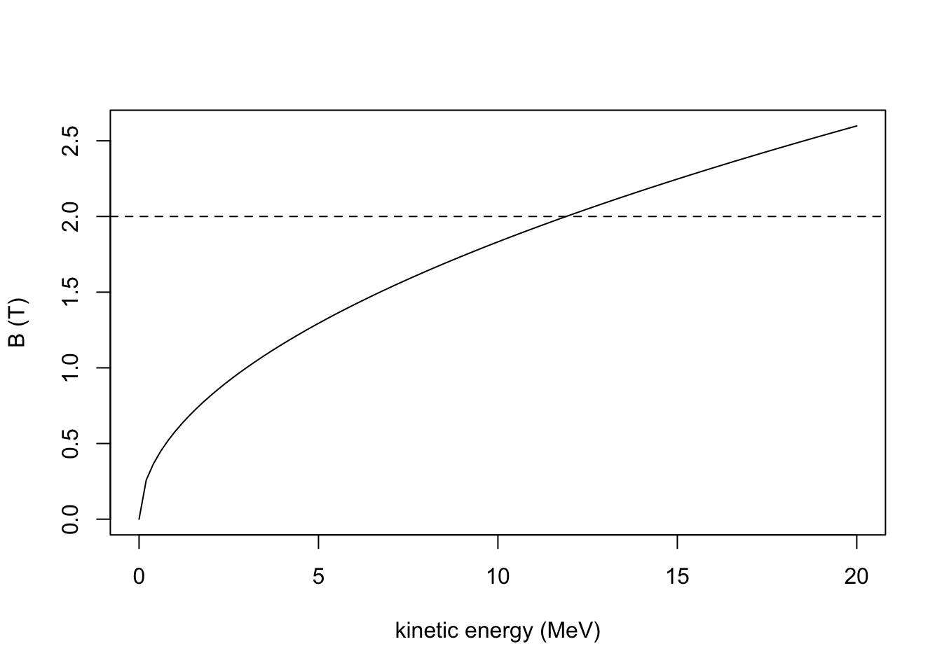
Homework Problem 2:
E0 = 0.511 # MeV
W = 200    # MeV
pc = sqrt(((W+E0)/E0)^2 - 1)*E0/1000 # GeV
Brho = 10/2.9979*pc   #  T-m
F = 4       # m
Leff = 0.2  # m
d = 0.6 # m- Consider a beam of electrons, each with kinetic energy 200 MeV. A quadrupole lens is used to focus this beam, with a focal length of 4 m. What magnetic gradient, \(B'\), is required if the effective length of the magnet is 0.2 m? Is a thin lens approximation justified for use in this situation?
# 1/F = G Leff / Brho
Grad = Brho/F/Leff
Grad   # T/m
## [1] 0.836045Leff/F## [1] 0.05ifelse(Leff/F < 0.1, "yes", "no")## [1] "yes"We wish to focus the beam both horizontally and vertically using a “doublet”. Consider a second quadrupole magnet with the same parameters as the one used above, but with its electrical polarity reversed creating a “defocusing” lens. If these two thin lenses are now separated by 0.6 m, center-to-center, with the beam passing through the horizontally focusing magnet first and then the horizontally defocusing magnet,
- what is the resulting focal length in the horizontal plane?
- What is it in the vertical plane?
- How do these compare with the theoretical thin lens doublet focal length?
- Can you create a system of these two magnets that has the same focal length in both planes? (Justify your answer.)
- what is the resulting focal length in the horizontal plane?
In the above, measure focal length from the mid-point between the two quadrupole magnets.
MF = matrix(c(  1,  0,
              -1/F, 1), nrow=2, ncol=2, byrow=TRUE)
Md = matrix(c(  1,  d,
                0,  1), nrow=2, ncol=2, byrow=TRUE)
MD = matrix(c(  1,  0,
               1/F, 1), nrow=2, ncol=2, byrow=TRUE)
x0 = array(c(1,0))
x0
## [1] 1 0Outx = MD %*% Md %*% MF %*% x0
Outy = MF %*% Md %*% MD %*% x0
Fx = d/2 - Outx[1]/tan(Outx[2])
Fy = d/2 - Outy[1]/tan(Outy[2])
Fx## [1] 22.95604Fy## [1] 30.95229F^2/d## [1] 26.66667r0 = 1.1
x0 = c(1,0,1,0)
Out = function(r){
MF = matrix(c( 1, 0, 0, 0,
-1/F, 1, 0, 0,
0, 0, 1, 0,
0, 0, 1/F, 1 ), nrow=4, ncol=4, byrow=TRUE)
Md = matrix(c( 1, d, 0, 0,
0, 1, 0, 0,
0, 0, 1, d,
0, 0, 0, 1 ), nrow=4, ncol=4, byrow=TRUE)
MD = matrix(c( 1, 0, 0, 0,
1/F*r, 1, 0, 0,
0, 0, 1, 0,
0, 0, -1/F*r, 1 ), nrow=4, ncol=4, byrow=TRUE)
MD %*% Md %*% MF %*% x0
}
Fcn = function(r){
V = Out(r)
Fx = d/2 - V[1]/tan(V[2])
Fy = d/2 - V[3]/tan(V[4])
abs(Fx-Fy)
}
F2d = optimize(Fcn,c(0.5,1.5))
rFin = F2d$minimumVf = Out(rFin)
Fx = d/2 - Vf[1]/tan(Vf[2])
Fy = d/2 - Vf[3]/tan(Vf[4])paste("Increase strength of D quad by factor ", round(rFin,4), ".")## [1] "Increase strength of D quad by factor 1.023 ."paste("Common focal length will be Fx =", round(Fx,2), "m, Fy = ", round(Fy,2), "m.")## [1] "Common focal length will be Fx = 26.35 m, Fy = 26.35 m."