6 Longitudinal Dynamics
Discussion Topics…
- Cavities
- Beam Bunching
- The Slip Factor
Difference Equations
- Synchrotron Motion
- Non-linear RF Bucket and The Standard Map
Bunch Manipulations
Homework Problem 1:
QonA = c(1/6,1/3,1/2,1)
mc2 = 931
eVup = 10   # MeV
eVdn = 0.05 # MeV- Generate a set of curves of \(\beta~(= v/c)\) vs. \(eV\) for values of \(Q/A =\) 0.167, 0.333, 0.5, 1, where 0.05 MeV \(< eV <\) 10 MeV. Here, \(eV\) is the kinetic energy per nucleon of a particle of charge \(Qe\) and rest energy \(A\mu\), where \(\mu\) = 931 MeV (the rest energy of a nucleon).
z=QonA[length(QonA)]
beta = function(x){ sqrt(1-(mc2/(mc2+x*z))^2) }
curve(beta,eVdn,eVup,
    xlab="eV [MeV]",ylab="v/c", main="Speed vs. Voltage, for various Q/A")
i=0
while(i<length(QonA)){
  z=QonA[length(QonA)-i]
  curve(beta,eVdn,eVup,
    lty=i+1,col=2*i+2,add=TRUE)
  i = i+1
}
text(9,c(0.045,0.075,0.105,0.130),c("1/6","1/3","1/2","1"))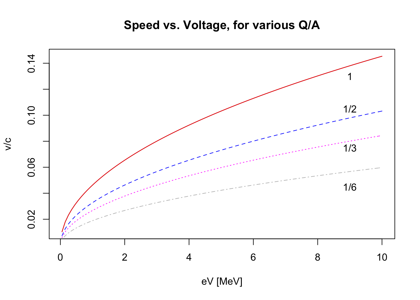
- Consider a set of 2-gap, \(\pi\)-mode accelerating cavities, each designed for an optimal velocity, \(\beta_{opt}\). (Assume constant \(E_z\), etc.) For each, assume the length of each gap is \(g = \beta_{opt}\lambda/8\), and the distance between gap centers is \(d = \beta_{opt}\lambda/2\). The transit time factor for a cavity is thus
\[ T(\beta) = \frac{\sin(\pi g/\beta\lambda)}{\pi g/\beta\lambda} \cdot \sin(\pi d/\beta\lambda). \]
c=2.9979e8
betOpt = c(0.041,0.085,0.29,0.53)
frf = c(80.5,80.5,322,322)*1e6
lambda = c/frf
gap = betOpt[1]*lambda[1]/8
d = gap*4
TTF = function(x){
  sin(pi*gap/x/lambda)/(pi*gap/x/lambda)*sin(pi*d/x/lambda)
}
Plot the transit time factors \(T(\beta)\) vs. \(\beta\) for the following 4 cases:
- for \(\lambda\) corresponding to 80.5 MHz,
- \(\beta_{opt}\) = 0.041, and
- \(\beta_{opt}\) = 0.085; and,
- for \(\lambda\) corresponding to 322 MHz,
- \(\beta_{opt}\) = 0.29, and
- \(\beta_{opt}\) = 0.53.
For each case, estimate the range of velocities for which the transit time factor is greater than 50%.
curve(0*x, 0.001, 0.75, ylim=c(-1.0,1.3),
  xlab="v/c", ylab="Transit Time Factor")
color = c("black","red","blue","brown")
i = 1
while(i<5){
  lambda = c/frf[i]
  gap = betOpt[i]*lambda/8
  d = gap*4
  TTF = function(x){
    sin(pi*gap/x/lambda)/(pi*gap/x/lambda)*sin(pi*d/x/lambda)
  }
  curve(TTF(x),0.001,0.75,col=color[i],add=TRUE)
  i = i+1
}
abline(h=0.50,lty=2)
abline(v=betOpt,lty=4)
text(betOpt,c(1.25,1.10,1.25,1.25),betOpt)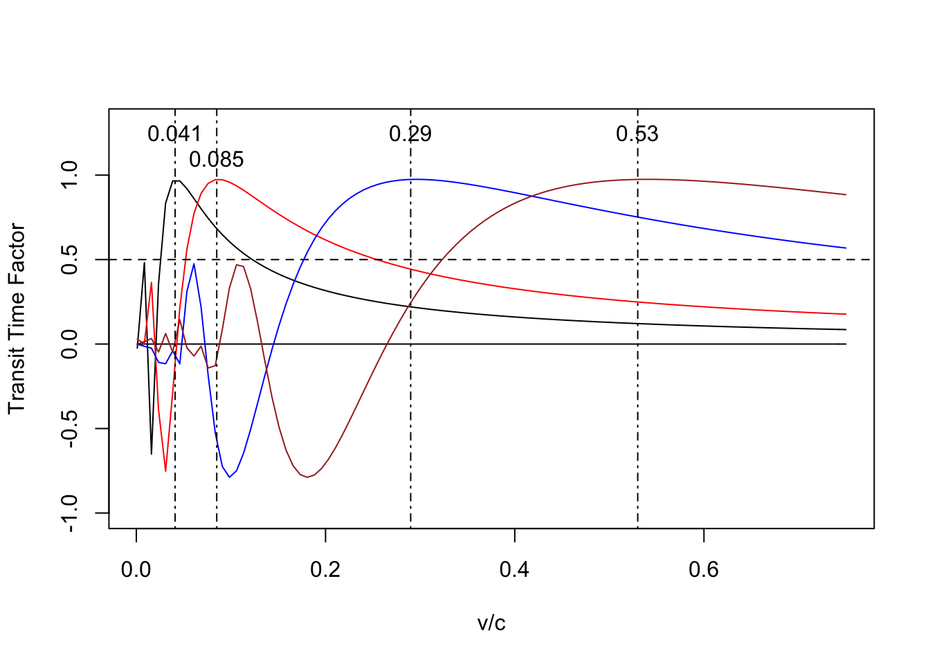
Homework Problem 2:
The area \({\cal A_0}\) of a “stationary bucket” (\(\phi_s\) = 0, \(\pi\) ) in \(\phi\)-\(\Delta E\) phase space is:
\[ {\cal A_0} = \frac{16\;v/c}{2\pi f_{RF}} \sqrt{\frac{eV\;E_s}{2\pi h |\eta|}} \]
For values of synchronous phase between 0 and 90\(^\circ\), create a curve of the area \({\cal A}\) of a “bucket” in units of \({\cal A_0}\).
For \(\phi_s\) between 0 and 90\(^\circ\) in steps of 2\(^\circ\), create a table of values for \(\phi_1\), \(\phi_2\), and \({\cal A}/{\cal A_0}\), where \(\phi_1\) and \(\phi_2\) are the phase limits for stable motion.
Xout <- array(0,dim=c(46,4))
phisDeg <- 0

i = 1
while (i<47){
  phisDeg = 2*(i-1)
  phis = phisDeg*pi/180

  f = function(x){
      cos(x) + x*sin(phis) + cos(phis) - (pi-phis)*sin(phis) }
  phi1 = uniroot( f, c(-pi,pi))$root
  phi2 = pi - phis

  dE <- function(x){
      sqrt( cos(x) + x*sin(phis) - cos(phi2) - phi2*sin(phis)) }

  A <- 1/4/sqrt(2)*integrate(dE, phi1, phi2)$value

  Xout[i,] = c(phis*180/pi, phi1*180/pi, phi2*180/pi, A)

  i = i+1
}

plot(Xout[,1],Xout[,4],typ="l", xlab="Synchronous Phase (deg)", ylab="A/A_0", xaxs="i", yaxs="i",ylim=c(0,1.1))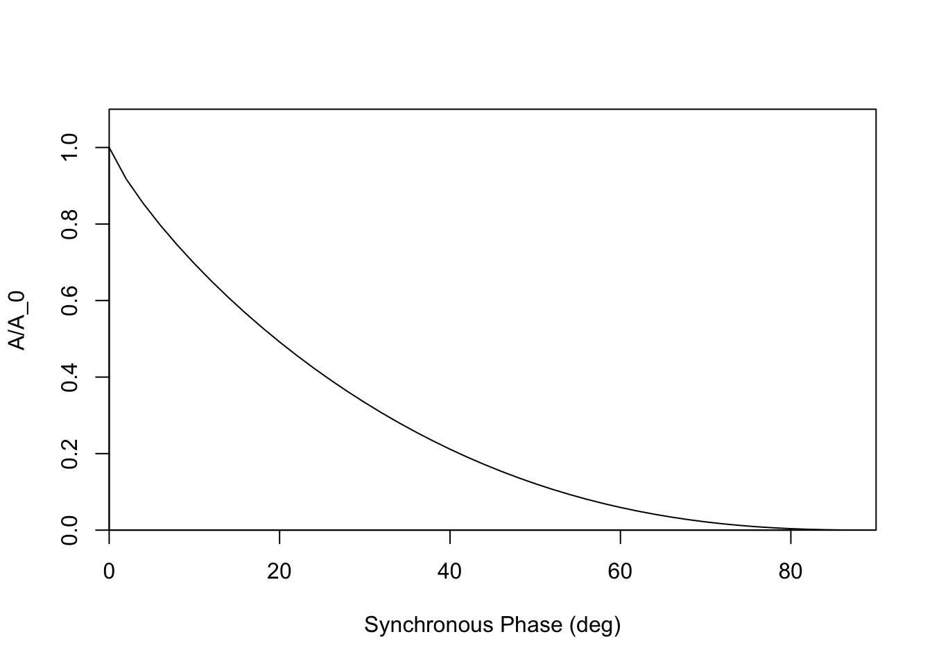
tableLabels = c("phis","phi1","phi2","area")
table1 = rbind(round(Xout,3))
colnames(table1) = tableLabels
print(table1,quote=FALSE)
## phis phi1 phi2 area
## [1,] 0 -180.000 180 1.000
## [2,] 2 -143.474 178 0.918
## [3,] 4 -128.791 176 0.854
## [4,] 6 -117.556 174 0.797
## [5,] 8 -108.060 172 0.745
## [6,] 10 -99.647 170 0.696
## [7,] 12 -91.990 168 0.651
## [8,] 14 -84.891 166 0.608
## [9,] 16 -78.227 164 0.567
## [10,] 18 -71.911 162 0.529
## [11,] 20 -65.879 160 0.492
## [12,] 22 -60.087 158 0.457
## [13,] 24 -54.496 156 0.424
## [14,] 26 -49.081 154 0.392
## [15,] 28 -43.817 152 0.362
## [16,] 30 -38.686 150 0.333
## [17,] 32 -33.673 148 0.306
## [18,] 34 -28.763 146 0.281
## [19,] 36 -23.947 144 0.256
## [20,] 38 -19.215 142 0.233
## [21,] 40 -14.558 140 0.212
## [22,] 42 -9.968 138 0.191
## [23,] 44 -5.441 136 0.172
## [24,] 46 -0.969 134 0.154
## [25,] 48 3.452 132 0.137
## [26,] 50 7.825 130 0.121
## [27,] 52 12.158 128 0.107
## [28,] 54 16.451 126 0.093
## [29,] 56 20.707 124 0.081
## [30,] 58 24.932 122 0.070
## [31,] 60 29.126 120 0.059
## [32,] 62 33.296 118 0.050
## [33,] 64 37.442 116 0.041
## [34,] 66 41.562 114 0.034
## [35,] 68 45.667 112 0.027
## [36,] 70 49.748 110 0.022
## [37,] 72 53.819 108 0.017
## [38,] 74 57.873 106 0.012
## [39,] 76 61.916 104 0.009
## [40,] 78 65.946 102 0.006
## [41,] 80 69.968 100 0.004
## [42,] 82 73.985 98 0.002
## [43,] 84 77.993 96 0.001
## [44,] 86 81.998 94 0.000
## [45,] 88 85.999 92 0.000
## [46,] 90 90.002 90 0.000Homework Problem 3:
E0 <- 938 # MeV
eV <- 4 # MeV
h <- 588
Es <- 8938 # MeV
gamt = 22
phis = 0
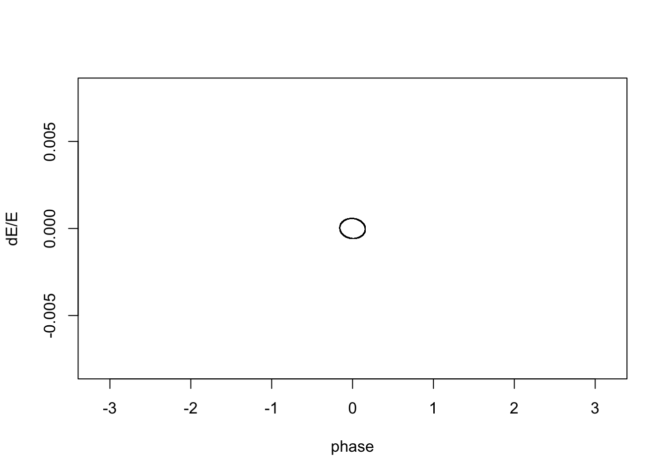
Nturns = 2^10 - 2Create a routine to track the longitudinal phase space motion (\(\phi_n\), \(\Delta E_n\)) of a proton in a synchrotron undergoing longitudinal oscillations within a “stationary bucket” (i.e., \(\phi_s=0\) for \(\gamma < \gamma_t\)) for a number of iterations, \(N\), where \(1<n<N\). Assume the proton starts with initial \(\Delta E_0\) = 0 and an initial phase \(\phi_0\) (say, \(\pi/20\)). Use the Fermilab Main Injector for our example, which has the following parameters:
- \(V\) = 4 MV; \(h\) = 588; \(E_s\) = 8938 MeV; \(\gamma_t\) = 22
Make a plot in \(\phi-\Delta E\) phase space of the particle motion over 1022 turns.
vonc = sqrt(1-(E0/Es)^2)
eta  = 1/gamt^2 - (E0/Es)^2
k    = 2*pi*h*eta/vonc^2
phi0 = pi/20

phi    = array(phi0, dim=Nturns)
dEonE  = array(0,    dim=Nturns)
dEonEmax = 0.008

plot(phi, dEonE, type="n", xlab="phase", ylab="dE/E",
   xlim=c(-pi,pi), ylim=c(-1,1)*dEonEmax, )

# track the particle...
for (j in 2:Nturns){
    du = dEonE[j-1] + eV/Es*(sin(phi[j-1])-sin(phis))
    dEonE[j] = du
    phi[j] = phi[j-1] + k*du
    if (phi[j] >  pi) { phi[j] = phi[j] - 2*pi }
    if (phi[j] < -pi) { phi[j] = phi[j] + 2*pi }
    if (dEonE[j] > dEonEmax*100) {dEonE[j] = 0  }
    points(phi[j], dEonE[j], type="p",pch=".")
}
R has a built-in Fast Fourier Transform (FFT) function that allows one to analyze data for frequency content. The frequency (or, in this case, the “synchrotron tune”) of the particle’s motion can be estimated by looking at what tune value corresponds to the peak of the FFT coefficients. The following is a code chunck that creates a function to perform an FFT on a set of data, and find the value of the peak coefficient:
# Fast Fourier analyze the data to extract a "tune"
fftpeak = function(x){
   zz_x = abs(fft(x))
   f_x  = c(1:length(x))/length(x)
   f_xfft = f_x[ max.col( t( cbind( f_x, zz_x) ) )[2] ]
   nu_x = min(f_xfft, (1-f_xfft))
   nu_x
}
Again, track a particle for 1022 turns (Note: FFT calculations often perform best when using \(2^N\) − 2 data points) which has initial conditions \(\phi_0 = \pi/20\) and \(\Delta E_0\) = 0.
- What synchrotron tune does an FFT analysis of the phase data (\(\phi_n\)) show? How does this compare with the analytically predicted value?
# Fast Fourier analyze the data to extract a "tune"
nu_u = fftpeak(phi)
nu_u
## [1] 0.018591nus_theory = sqrt(h*abs(eta)*eV*cos(phis)/(2*pi*vonc^2*Es))
nus_theory## [1] 0.0194653- Try varying the number of turns tracked, such as 510, 2046, 4094, etc. For what number of turns is the FFT result within 5% of the predicted result?
Na = 2^c(9,10,11,12,13) - 2

phi    = array(phi0, dim=Nturns)
dEonE  = array(0,    dim=Nturns)

nus_theory = sqrt(h*abs(eta)*eV*cos(phis)/(2*pi*vonc^2*Es))
print(paste("theoretical nu_s = ",round(nus_theory,4)))
## [1] "theoretical nu_s = 0.0195"# track the particle...
Nturns = Na[1]
for (i in 1:length(Na)){
phi[1] = phi0
dEonE[1] = 0
for (j in 2:Nturns){
du = dEonE[j-1] + eV/Es*(sin(phi[j-1])-sin(phis))
dEonE[j] = du
phi[j] = phi[j-1] + k*du
}
nu_u = fftpeak(phi)
print(paste("For ", Nturns, " turns, nu_u = ",round(nu_u,5)))
print(paste(" dnu/nu = ",
round(abs(nu_u-nus_theory)/nus_theory*100,2)," %"))
Nturns = Na[i+1]
}## [1] "For 510 turns, nu_u = 0.00098"
## [1] " dnu/nu = 94.97 %"
## [1] "For 1022 turns, nu_u = 0.02055"
## [1] " dnu/nu = 5.56 %"
## [1] "For 2046 turns, nu_u = 0.01906"
## [1] " dnu/nu = 2.07 %"
## [1] "For 4094 turns, nu_u = 0.0193"
## [1] " dnu/nu = 0.87 %"
## [1] "For 8190 turns, nu_u = 0.01954"
## [1] " dnu/nu = 0.36 %"- Next, to get an accurate result, track a particle through 16382 turns. Track for various initial \(\phi_0\)’s from \(10^\circ\) toward \(180^\circ\) and keep track of the synchrotron tune. How does the tune behave? Make a plot of \(\nu_s\) vs. \(\phi_0\) for the range within the stable region (separatrix).
Nturns = 2^14-2
phi_init = c(1:18)*10*pi/180

phi    = array(pi/10, dim=Nturns)
dEonE  = array(0,     dim=Nturns)
tune   = array(0,     dim=length(phi_init))
# track the particle...
phi0 = phi_init[1]
for (i in 1:length(phi_init)){
  phi[1]   = phi0
  dEonE[1] = 0
  for (j in 2:Nturns){
      du = dEonE[j-1] + eV/Es*(sin(phi[j-1])-sin(phis))
      dEonE[j] = du
      phi[j] = phi[j-1] + k*du
    }
  nu_u = fftpeak(phi)

  print(paste("For phi_0 = ", phi0*180/pi, ", nu_u = ",round(nu_u,6)))

  tune[i] = nu_u
  phi0 = phi_init[i+1]
}
## [1] "For phi_0 = 10 , nu_u = 0.019351"
## [1] "For phi_0 = 20 , nu_u = 0.019412"
## [1] "For phi_0 = 30 , nu_u = 0.019106"
## [1] "For phi_0 = 40 , nu_u = 0.018801"
## [1] "For phi_0 = 50 , nu_u = 0.018496"
## [1] "For phi_0 = 60 , nu_u = 0.018069"
## [1] "For phi_0 = 70 , nu_u = 0.01758"
## [1] "For phi_0 = 80 , nu_u = 0.017031"
## [1] "For phi_0 = 90 , nu_u = 0.016543"
## [1] "For phi_0 = 100 , nu_u = 0.015749"
## [1] "For phi_0 = 110 , nu_u = 0.015078"
## [1] "For phi_0 = 120 , nu_u = 0.014223"
## [1] "For phi_0 = 130 , nu_u = 0.013307"
## [1] "For phi_0 = 140 , nu_u = 0.01227"
## [1] "For phi_0 = 150 , nu_u = 0.010988"
## [1] "For phi_0 = 160 , nu_u = 0.009767"
## [1] "For phi_0 = 170 , nu_u = 0.008058"
## [1] "For phi_0 = 180 , nu_u = 6.1e-05"plot(phi_init,tune)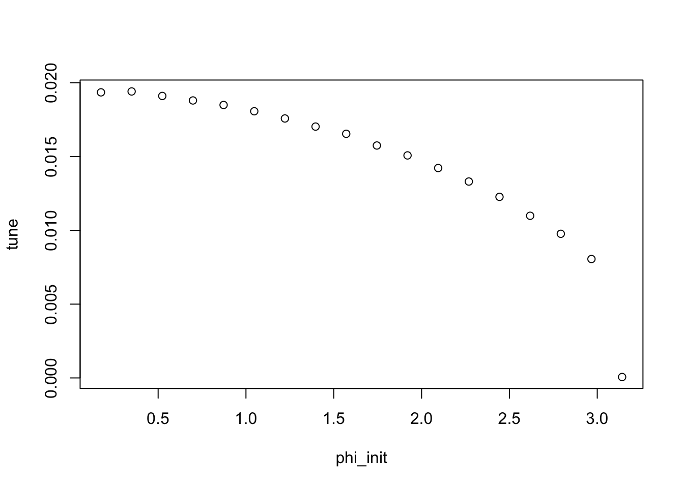
- What can you say about the particle motion on or very near the separatrix?
Homework Problem 4:
C = 6000    # m
h = 1100
gamt = 18
gam = 1000
dz = 0.027  # m
Dx = 5.2    # m
dR = 0.0005  # m
Two bunched beams of protons are counter-circulating in a synchrotron collider and are being brought into collision. Initially these bunches have identical average momentum, \(p_0\). The detector system shows that collisions are occuring, but the maximum of the luminosity is located 27 mm from the center of the detector and this needs to be corrected. Using an RF cavity system, the momentum of one beam relative to its initial momentum is increased by fraction \(\delta = \Delta p/p_0\), while the other beam has its average momentum held steady. The RF systems operate at a harmonic number of \(h\) = 1100 in the collider which has a circumference of 6 km. The transition energy of the synchrotron is at \(\gamma_t\) = 18 while the operation is performed at high energy where \(\gamma\) = 1000.
- A Beam Position Monitor is located where the horizontal dispersion is 5.2 m. If a 0.5 mm change in the radial position (in magnitude) is observed during the operation, what relative change in momentum \(\delta\) does this correspond to?
del = dR/Dx
del
## [1] 9.615385e-05- Assuming this change in momentum is made instantaneously, approximately how many revolutions about the synchrotron must the particles make before the collisions can become centered in the detector? How long does this take?
# dt/T = eta dp/p = eta * del
# n * dt * v = dz
# so, n = dz/(dt*v) = dz/(T*v*eta*del) = dz/(C*eta*del)
eta = 1/gamt^2-1/gam^2
n = dz/C/eta/del
floor(n)
## [1] 15#Note:
v = 3e8*sqrt(1-1/gam^2)
n*C/v*1e3 # time, milliseconds (for v = c)## [1] 0.3033624- What change in the RF frequency (magnitude) is required to implement this operation?
# df/f = - eta * del
# f_RF = h*f_rev = h*v/C;  so, ...
df_RF = -h*v/C*eta*del
abs(df_RF)  # Hz
## [1] 16.31712