C Getting to Know R
For solutions to various exercises involved in the class and for general computations performed in the lectures and throughout these notes, the statistical programming language R has been used. (R Core Team 2016) This programming environment (a) is available on all major platforms (Mac, PC, unix, linux), (b) has many easy-to-use (and many not-so-easy-to-use) built-in functions for plotting data, generating curves, manipulating matrices, etc., and best of all (c) is freely available for download over the internet.
After installing R (and, perhaps, Rstudio) on your system and initializing,
- in the Console window, type commands and hit Return:
34 + 17## [1] 51sqrt(49)## [1] 7besselI(0.25,1)## [1] 0.1259791pi## [1] 3.141593- in the Source window, select lines that you wish to execute and (a) hit Run, or (b) hit Command-Return (MAC) or Control-Return (PC)
- if have a text file located in a directory /dir/filename that contains R commands, can type
source("/dir/filename")(quotation marks must be included) in the console window and hit Return to execute the commands.
C.1 Doing Simple Calculations
Define variables and perform calculations…
E0 = 938; W = 8000
sqrt( 1 - (E0/(E0+W))^2 )
## [1] 0.994478# or, define a variable:
beta = sqrt( 1 - (E0/(E0+W))^2 )
# just typing the name of the variable displays its value:
beta## [1] 0.994478Create a function as follows:
beta = function(x){ sqrt( 1 - (E0/(E0+x))^2 ) }
beta(8000)
## [1] 0.994478Make a list of numbers and perform a calculation on all of them
x = c(0,2,5,9,23)
beta(x)
## [1] 0.0000000 0.0651981 0.1028413 0.1375393 0.2174718Round off our answers to 3 digits
round(beta(x),3)## [1] 0.000 0.065 0.103 0.138 0.217C.2 Making Simple Plots
x = c(0,1,2,3,4,5,6,7,8,9)
y = beta(x)
plot(x,y)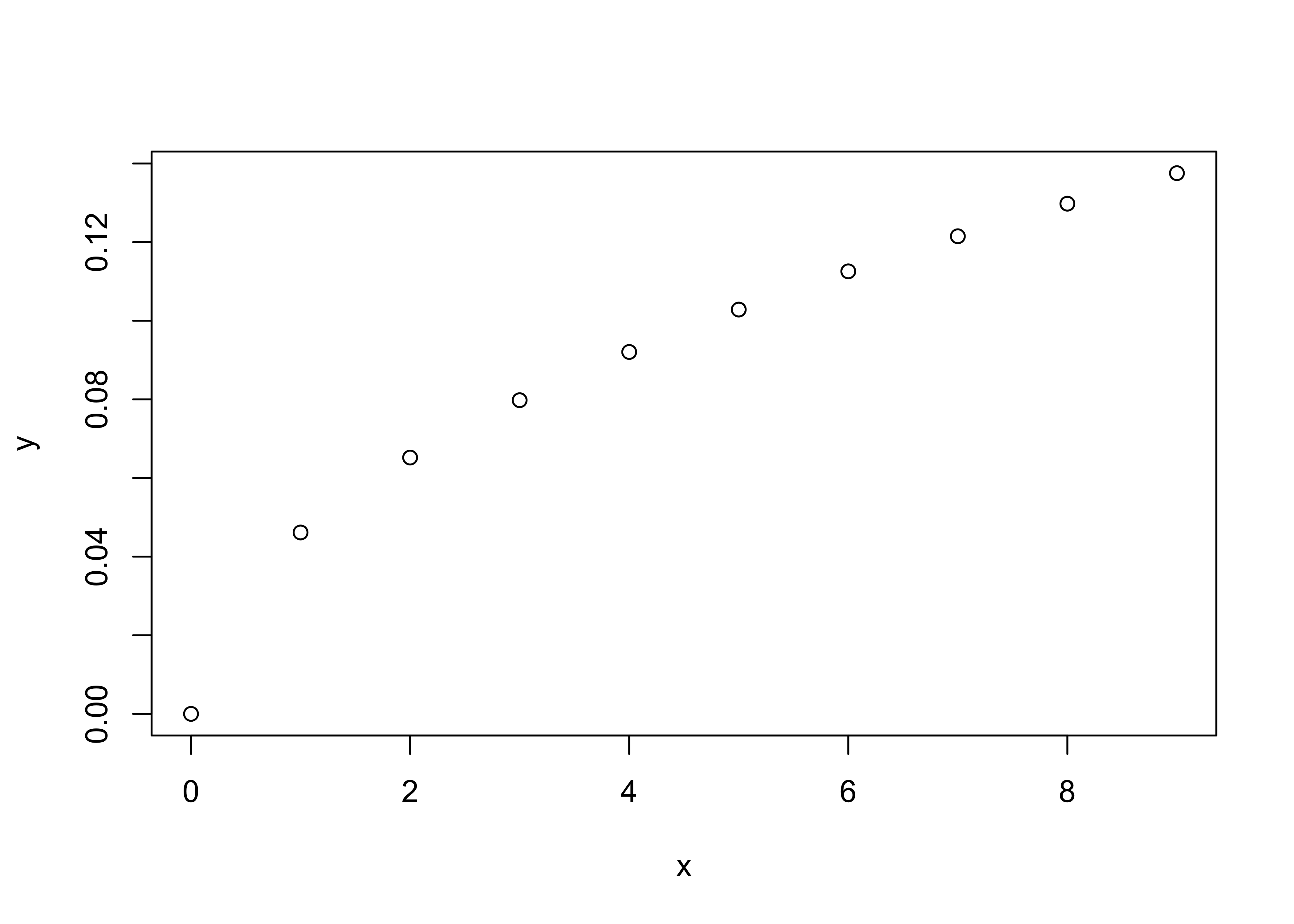
Plot a curve of a function
curve(beta,0,10)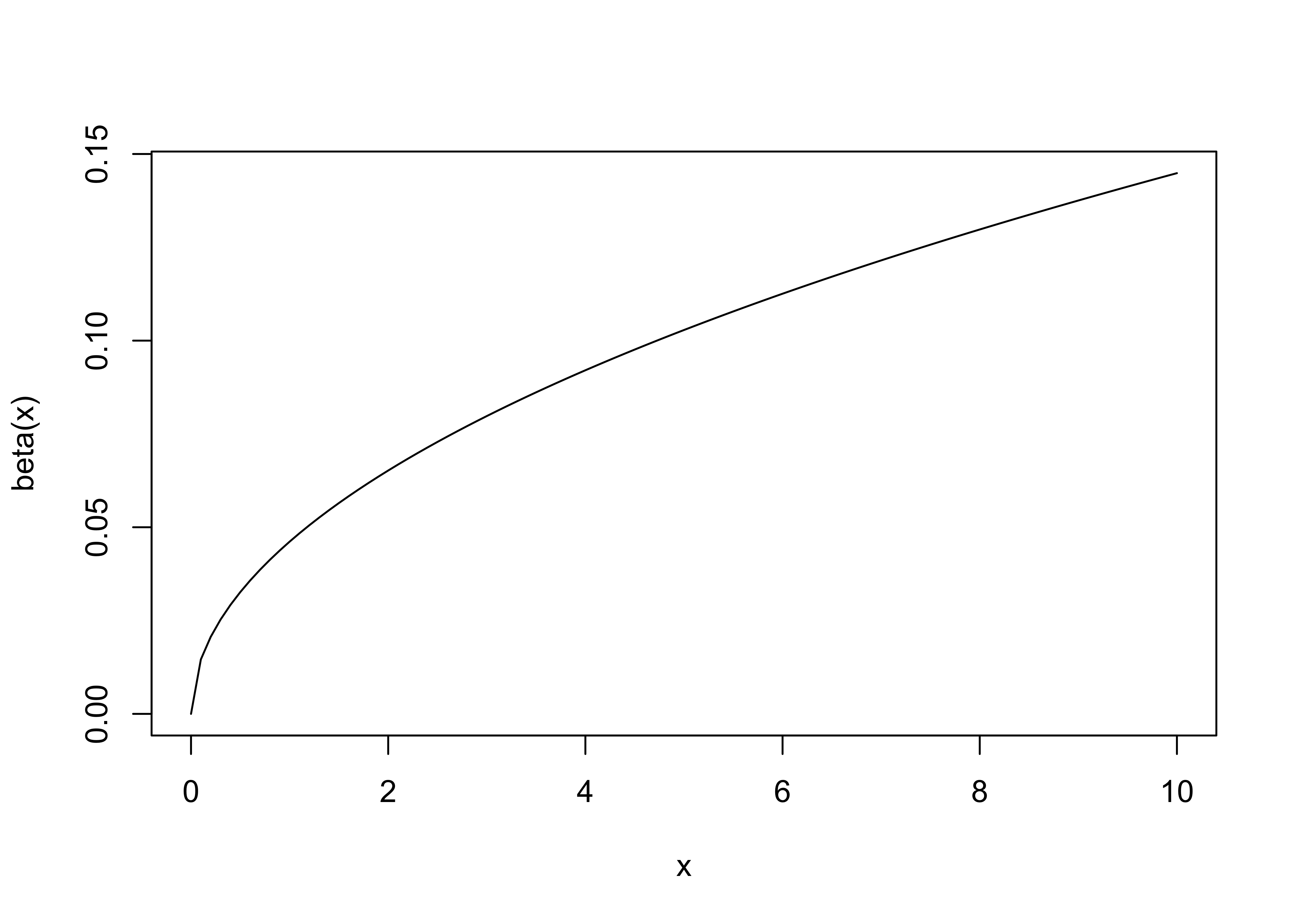
Plot the points, and add a curve to the same plot; also, add some new labels to the axes
plot(x,y,
   xlab="proton kinetic energy [MeV]", ylab="v/c", main="Velocity vs. Kinetic Energy")
curve(beta, 0, 10, add=TRUE, col="blue")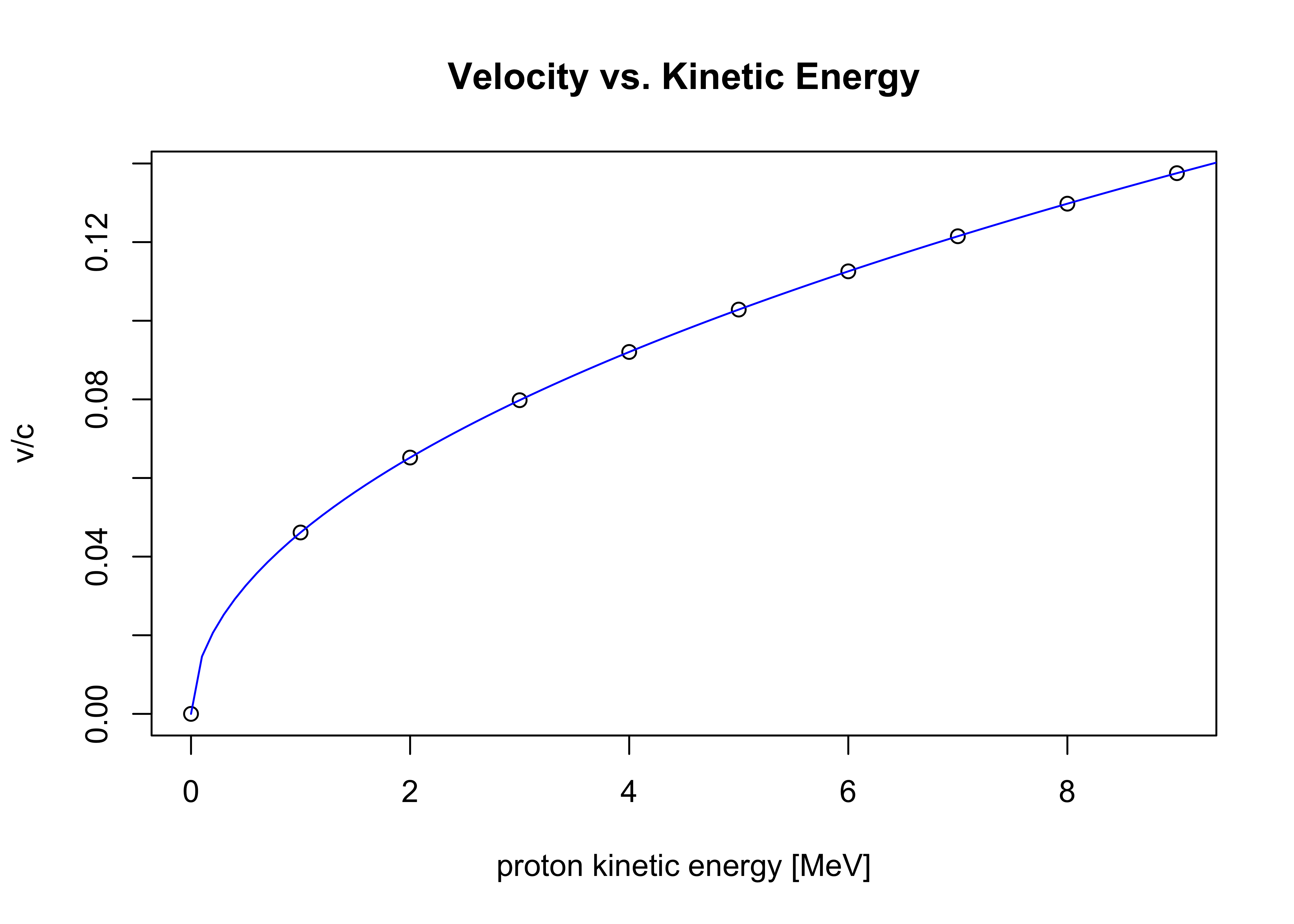
C.3 Creating Random Distributions
# Uniform Distribution of Npts points between 0 and 1
Npts = 500
r = runif(Npts,0,1)
plot(r)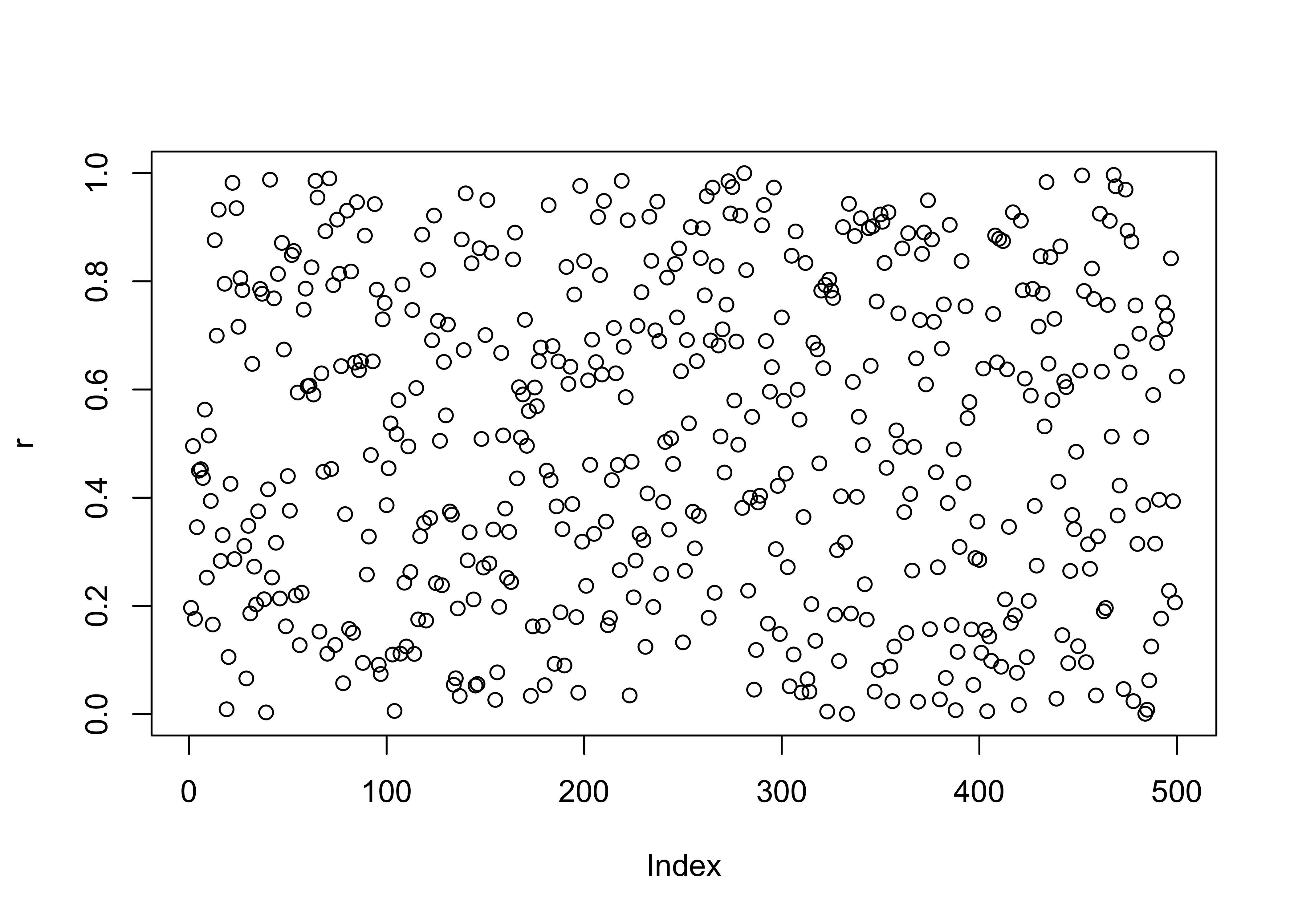
hist(r)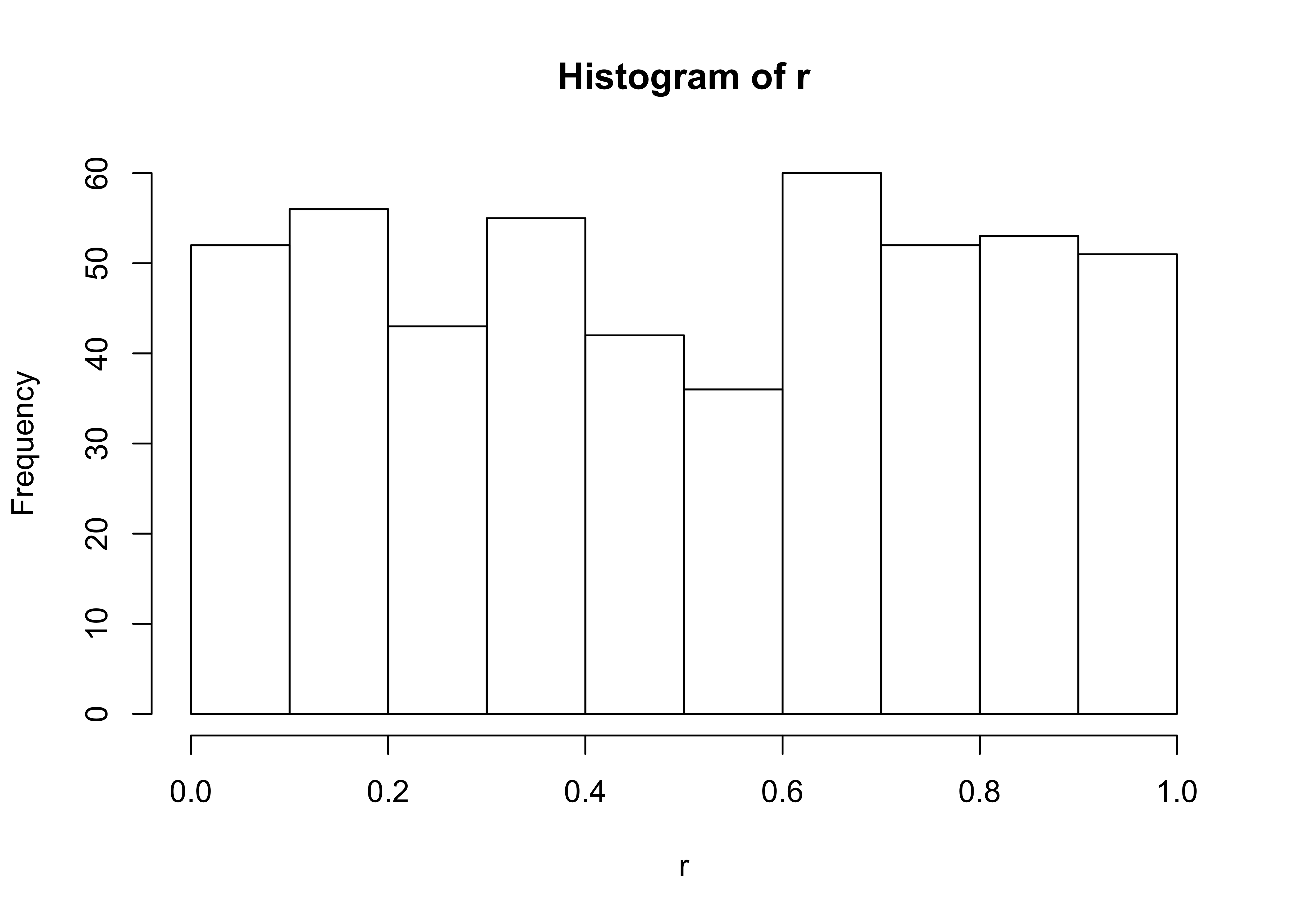
# Normal (Gaussian) Distribution of Npts points, with mean=0, sigma=sig
sig=2
set.seed(231)  # set the random number seed to get same results each run
r = rnorm(Npts,0,sig)
plot(r)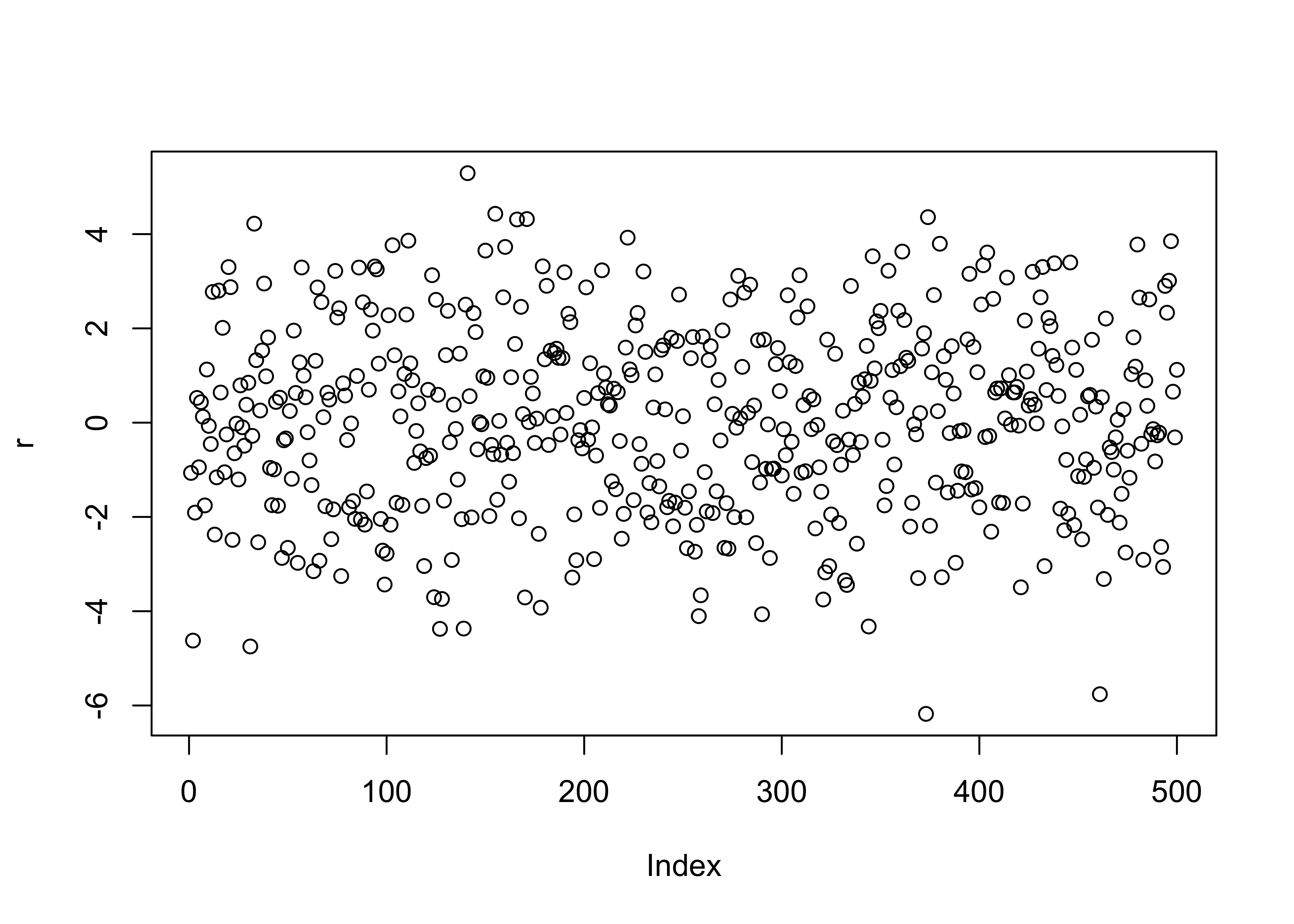
hist(r)
curve(Npts/(sqrt(2*pi)*sig)*exp(-x^2/(2*sig^2)), add=TRUE, col="blue")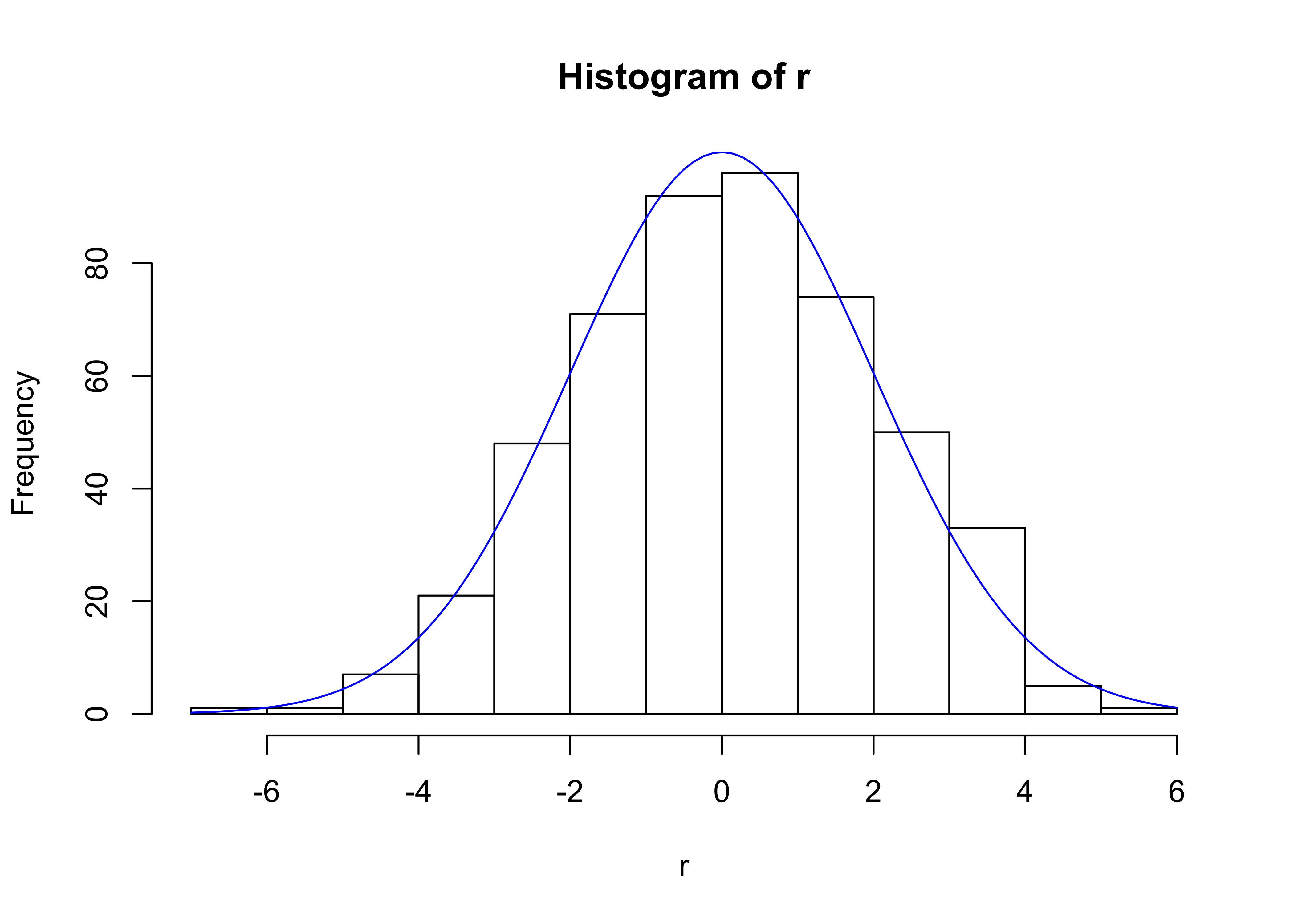
C.4 Decisions and Loops
imax=10
x = array(c(1:imax))
x
## [1] 1 2 3 4 5 6 7 8 9 10i = 1
while (i<imax){
x[i+1] = x[i] + 12
i = i+1
}
x## [1] 1 13 25 37 49 61 73 85 97 109Can use ifelse(test,yes,no) to perform tests and make decisions
imax=10
x = runif(imax,-1,1)
round(x,2)
## [1] -0.17 0.29 -0.56 0.82 -0.32 -0.25 -0.25 0.24 -0.70 0.50i = 1
while (i<imax+1){
x[i] = ifelse(x[i]<0, abs(x[i]), x[i])
i = i+1
}
round(x,2)## [1] 0.17 0.29 0.56 0.82 0.32 0.25 0.25 0.24 0.70 0.50C.5 Matrix Manipulations
A matrix is essentially an ordered list; so, create a list of numbers and tell R where to break the list into rows or columns.
M = matrix( c(1,2,3,4), ncol=2, byrow=TRUE)
M
## [,1] [,2]
## [1,] 1 2
## [2,] 3 4Nice to type the input this way, to visually emphasize the arrangement:
A = matrix( c(1, 2,
              3, 4  ), ncol=2, byrow=TRUE)
A
## [,1] [,2]
## [1,] 1 2
## [2,] 3 4B = matrix( c(5, 6,
7, 8 ), ncol=2, byrow=TRUE)
B## [,1] [,2]
## [1,] 5 6
## [2,] 7 8Multiply matrices – but be careful! If you write A * B, this will take each element of A (say a11) and multiply by the corresponding element in B (say b11). What we want is a real matrix multiply – performed using the %*% operator:
C = A * B
C
## [,1] [,2]
## [1,] 5 12
## [2,] 21 32WRONG!!
Here’s the right way (in R ):
C = A %*% B
C
## [,1] [,2]
## [1,] 19 22
## [2,] 43 50Take the transpose using t(), determinant using det()
t(A)## [,1] [,2]
## [1,] 1 3
## [2,] 2 4det(A)## [1] -2To find the inverse of a matrix, we use the solve() function:
solve(A)## [,1] [,2]
## [1,] -2.0 1.0
## [2,] 1.5 -0.5Check:
A %*% solve(A)## [,1] [,2]
## [1,] 1 1.110223e-16
## [2,] 0 1.000000e+00solve(A) %*% A## [,1] [,2]
## [1,] 1 4.440892e-16
## [2,] 0 1.000000e+00The function solve(A,B) solves the equation \(A\vec{x} = B\) for \(\vec{x}\). If \(B\) is missing in the solve() command, it is taken to be the identity and the inverse of \(A\) is returned. If you don’t like all the extra digits above, try:
round(solve(A) %*% A, 10)## [,1] [,2]
## [1,] 1 0
## [2,] 0 1Multiply a vector by a matrix to get a new vector; still use the operator %*%…
x = c(2,1)
x
## [1] 2 1t(t(x)) # trick, to see it in a "usual" (up/down) vector format## [,1]
## [1,] 2
## [2,] 1A## [,1] [,2]
## [1,] 1 2
## [2,] 3 4A %*% x## [,1]
## [1,] 4
## [2,] 10C.6 Reading/Writing Data
Write a set of numbers to a file, and read them back in…
x = rnorm(12,3,6)
y = rnorm(12,0,1)
write(c(x,y), file="data.txt", ncol=2)

data = scan("data.txt", list(0,0))
xx = data[[1]]  # first column
yy = data[[2]]  # second column

xx
## [1] 10.7197700 -6.8600400 0.8744534 5.4433470 3.1205390 4.8517960
## [7] 0.5321458 0.3883304 0.2311200 0.8316692 -1.6179690 -0.9675675yy## [1] -5.73622100 -3.83947800 6.52960600 11.36549000 -7.35074600
## [6] -4.79439500 0.02087685 -2.39514300 -0.16329580 0.85470720
## [11] -0.81268090 -0.97350320plot(xx,yy)
abline(h=mean(yy), v=mean(xx), lty=2)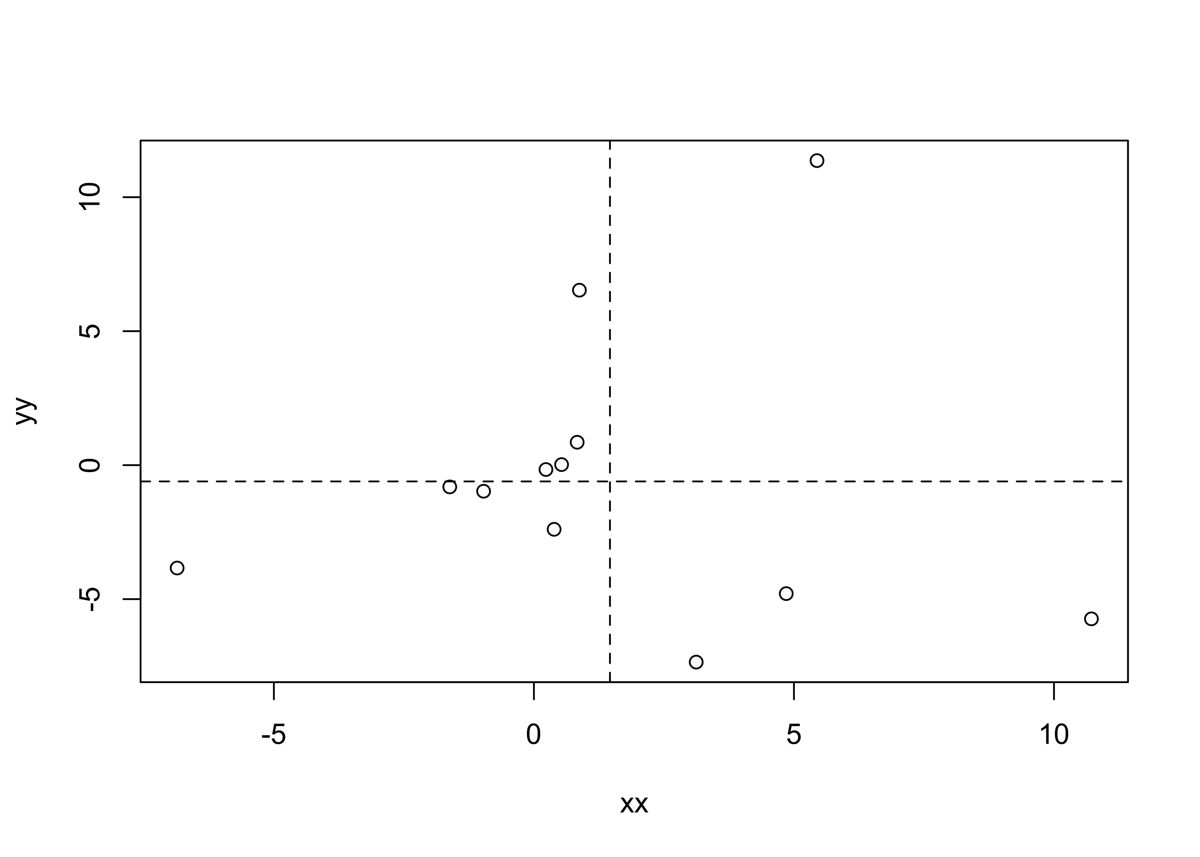
Note: The abline() function adds either horizontal, vertical, or general (\(y = a + bx\)) lines to an existing plot. The argument “typ” depicts the style of the line (solid, dotted, etc.).
C.7 Dataframes
Often times we wish to create or maybe read in a table of data, perhaps from measurements that were taken or from the results of a computer simulation, and take a quick look at the numbers, make simple plots, or pursue other manipulations. Above we read in data from a file and then identified new variables for each of the two columns of numbers. Below we will generate a new file of data and read it in using the read.table command; this will create a “dataframe” in R which makes many new options available for our use.
# Create some sample data and write to a file, with a header line
x = rnorm(50,0,2)
y = rnorm(50,0,5)
p = (y/5*2-5*x)/10
z = 2-(x+runif(50,-2,2))/2

filename = "data2.txt"
write(c("x","y","z","dp"), file=filename, ncol=4) # creates the file header
write(c(x,y,z,p), file=filename, ncol=4,append=TRUE) # writes the data
Next, we read the file back in, creating a dataframe named “data”.
filename = "data2.txt"
data = read.table(file=filename,header=TRUE,sep="")
# What have we created?
attributes(data)
## $names
## [1] "x" "y" "z" "dp"
##
## $class
## [1] "data.frame"
##
## $row.names
## [1] 1 2 3 4 5 6 7 8 9 10 11 12 13 14 15 16 17 18 19 20 21 22 23
## [24] 24 25 26 27 28 29 30 31 32 33 34 35 36 37 38 39 40 41 42 43 44 45 46
## [47] 47 48 49 50head(data) # look at first few lines of the dataframe## x y z dp
## 1 -0.6493544 0.7815001 2.5762840 -3.19092700
## 2 2.4029470 -0.7597306 0.7130670 2.75397700
## 3 1.1463000 2.5968690 -0.3912998 -3.37695700
## 4 0.8247087 2.1915740 -2.5770390 0.56283110
## 5 -1.7330390 -0.6709871 0.9480144 1.55270600
## 6 -0.5545588 -0.6730781 -1.4572720 0.07911138Note that the names of the columns in our dataframe are taken from the header (first line) of the text file we read in. To access the data for one of the variables (columns) from our dataframe data we use the dollar sign:
length(data$x) # number of entries for "x"## [1] 50data$x[23] # value of 23rd entry for "x"## [1] 4.047663print(sqrt(abs(data$x))) # perform calculation on all values of "x"## [1] 0.8058253 1.5501442 1.0706540 0.9081347 1.3164494 0.7446870 1.9749873
## [8] 1.1342077 1.1255052 1.1896802 1.4891138 0.8012527 0.6287553 1.9446804
## [15] 2.0392432 2.9948786 0.2325219 1.5465358 0.7394100 2.7627903 2.7006677
## [22] 1.3100065 2.0118805 2.5120924 2.6883102 1.1531383 0.4172762 0.7371416
## [29] 0.8368607 1.7644141 1.5815496 2.1275578 0.8835635 1.2090136 0.8348361
## [36] 1.5385493 1.4042486 1.3885503 1.1997554 0.4361112 0.7445951 1.1341768
## [43] 0.6150905 0.8663169 0.6248227 0.8470314 0.3659656 0.6364512 0.4919104
## [50] 1.0289198pairs(data) # create plots of each varialble vs. every other variable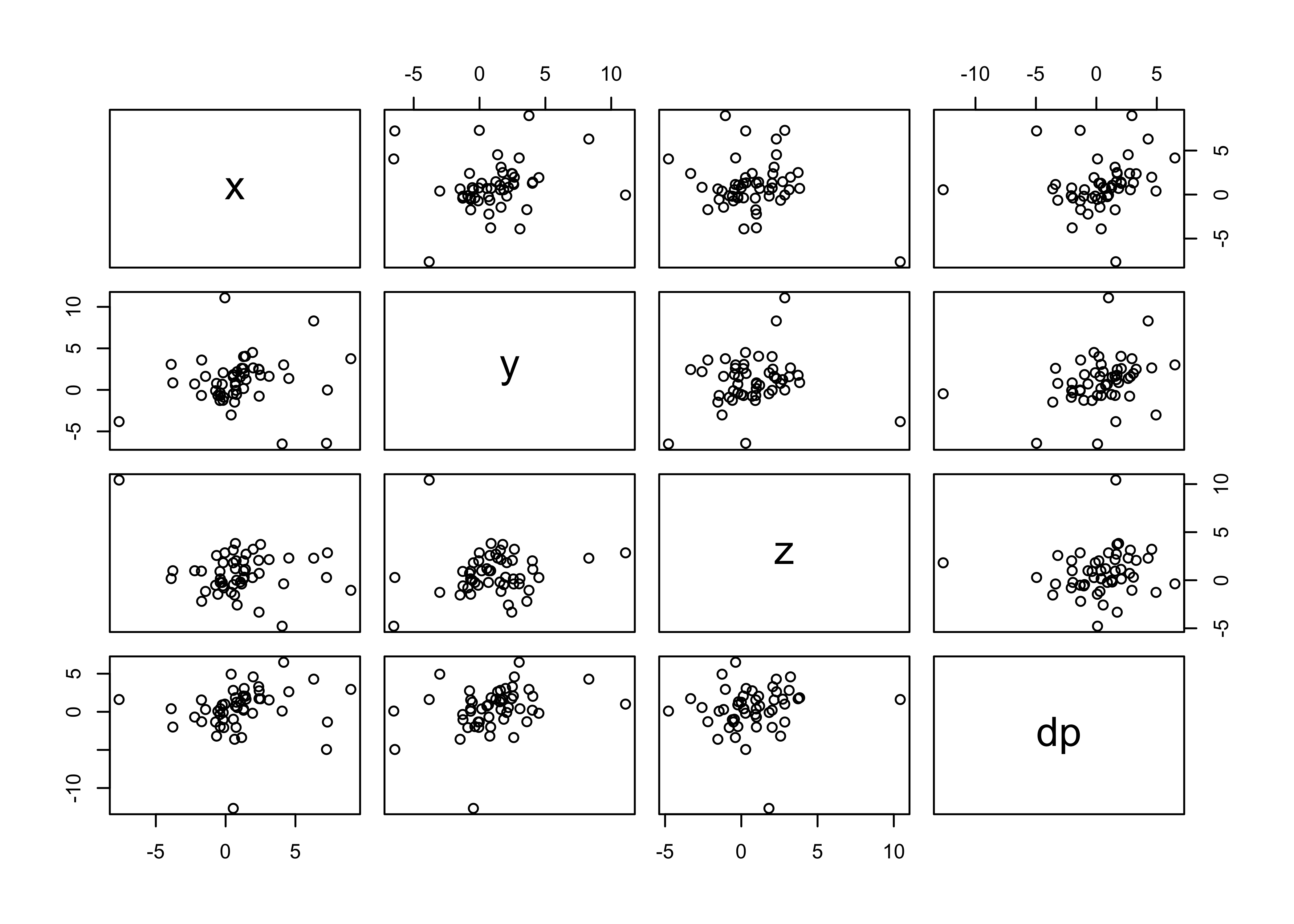
plot(data$x,data$dp) # plot one variable vs. another variable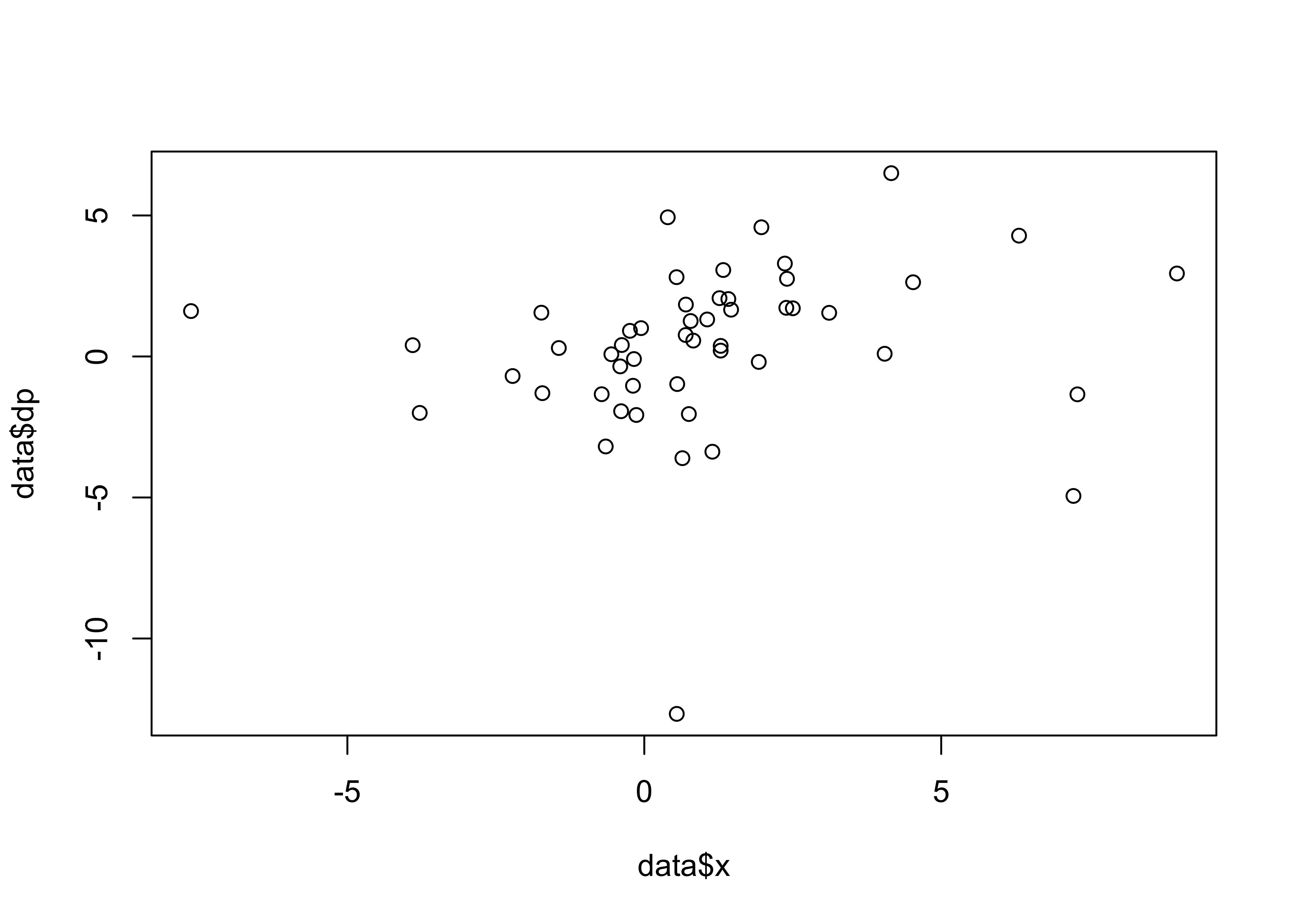
You can create a subsest of your dataset:
# find subset where abs(x)<0.8 AND abs(y)<1:
data_sub = subset(data, subset=( (abs(data$x)<4) & (abs(data$y)<1)) )
length(data_sub$x)
## [1] 17plot(data_sub$x,data_sub$dp) # plot one variable vs. another variable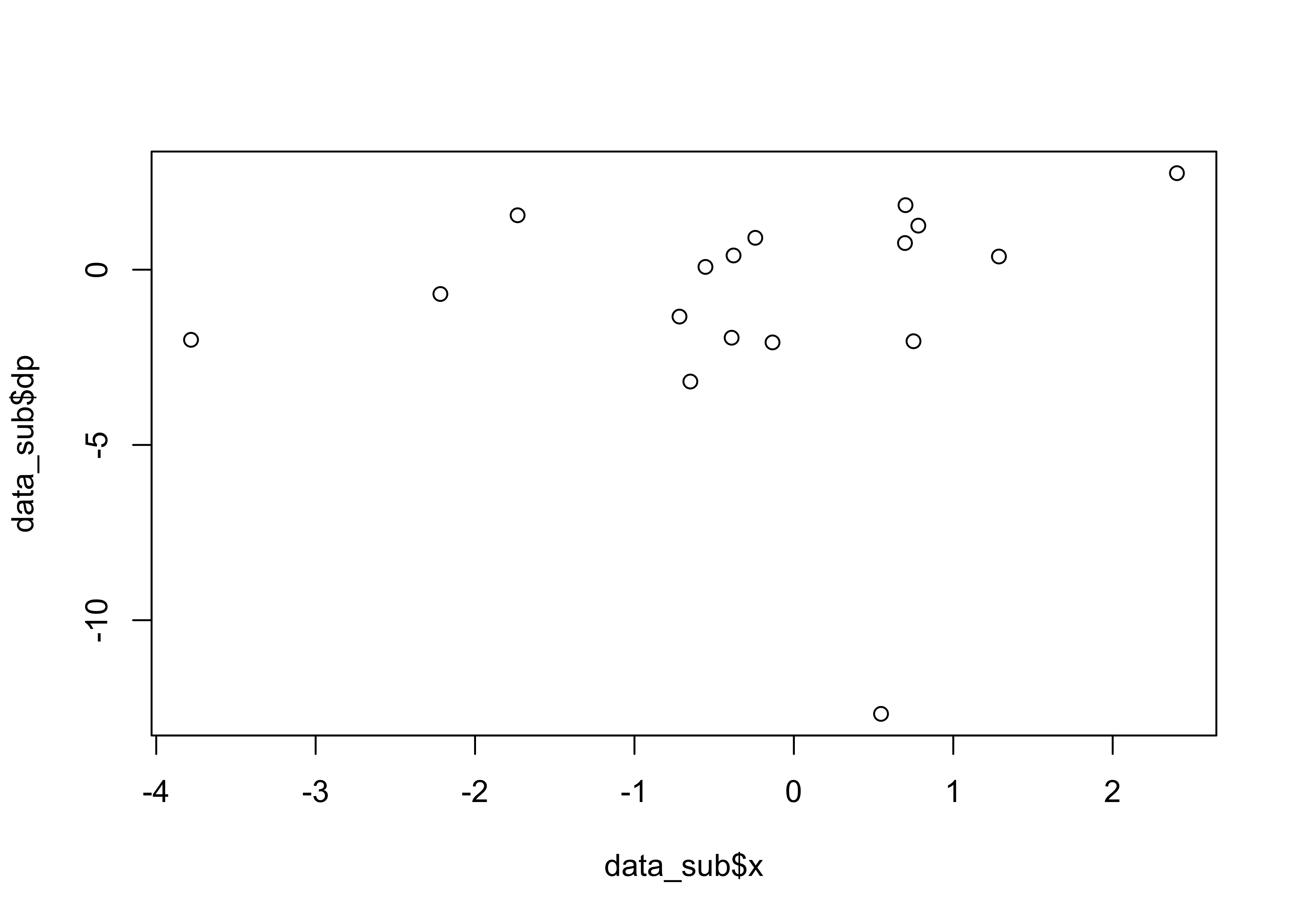
#  note: a & b     "a is true AND b is true" (intersection)
#        a | b     "a is true OR  b is true"    (union)
#         !a            "a is NOT true"        (negation)
#      other logical options:  a< b  a<=b  a==b  a>=b   a!=b
Next, we take our plot and fit the data to a linear model, finding the intercept and slope, and adding the corresponding line to the plot
fitparams = lm(dp ~ x, data_sub)
fitparams
##
## Call:
## lm(formula = dp ~ x, data = data_sub)
##
## Coefficients:
## (Intercept) x
## -0.8898 0.2453plot(data_sub$x,data_sub$dp)
abline(a=fitparams$coef[1], b=fitparams$coef[2],lty=2,col="red")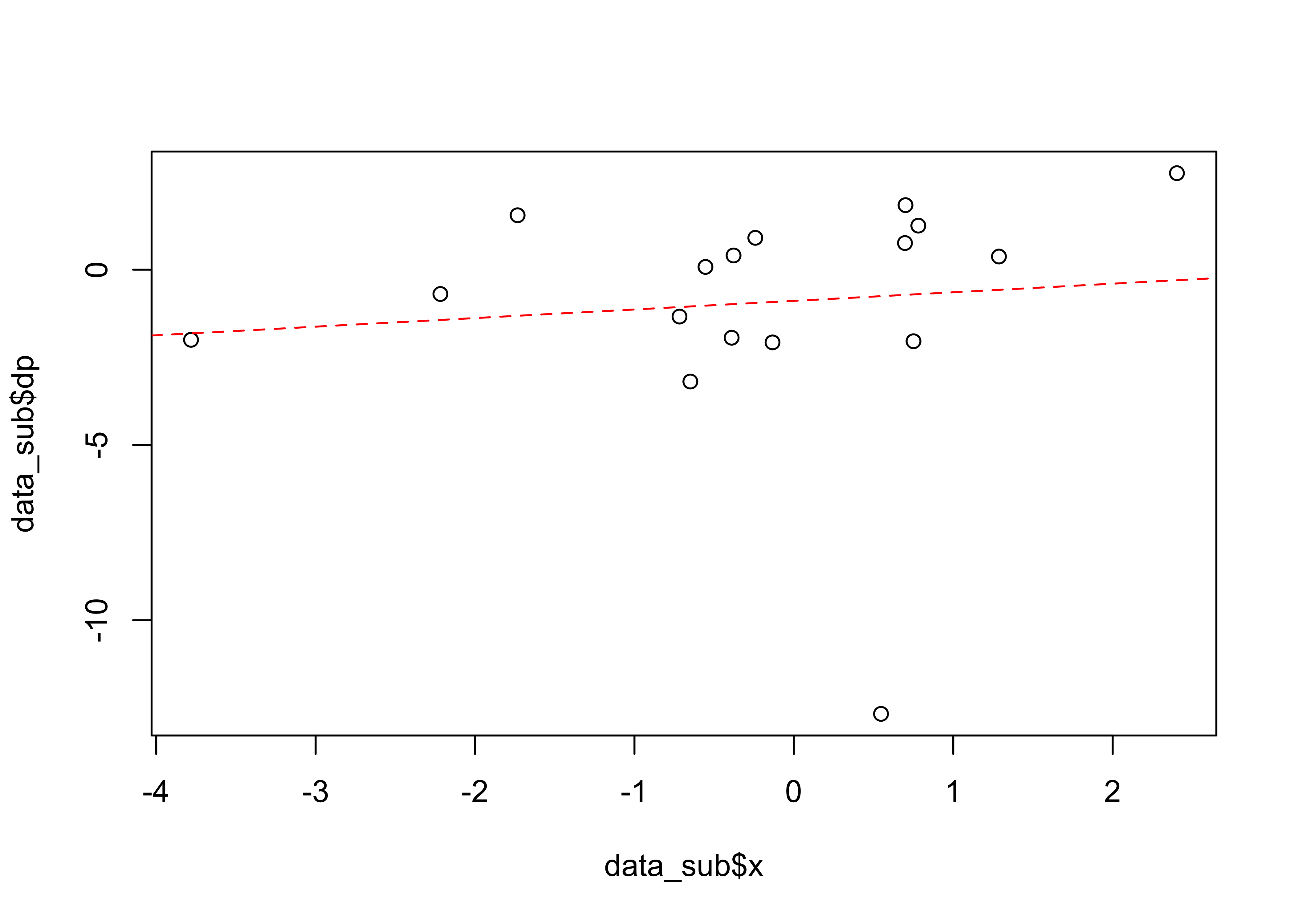
C.8 And Much, Much … Much, Much More
text manipulations; complex plotting control; optimizations; complex statistical analyses and modeling; …
visit: https://www.r-project.org/ for more information.
References
R Core Team. 2016. R: A Language and Environment for Statistical Computing. Vienna, Austria: R Foundation for Statistical Computing. https://www.R-project.org/.