A - Getting to Know R

Install and initialize R or Rstudio.

• in the Console window, type commands and hit Return:

34 + 17

## [1] 51

sqrt(49)

## [1] 7

besselI(0.25,1)

## [1] 0.1259791

pi

## [1] 3.141593

• in the Source window, select lines that you wish to execute and (a) hit Run, or (b) hit Command-Return (MAC) or Control-Return (PC)
• if have a text file located in a directory /dir/filename that contains R commands, can type source("/dir/filename") (quotation marks must be included) in the console window and hit Return to execute the commands.

A.1 Doing Simple Calculations

Define variables and perform calculations…

E0 = 938; W = 8000
sqrt( 1 - (E0/(E0+W))^2 )

## [1] 0.994478

# or, define a variable:
beta = sqrt( 1 - (E0/(E0+W))^2 )
# just typing the name of the variable displays its value:
beta

## [1] 0.994478

Create a function as follows:

beta = function(x){ sqrt( 1 - (E0/(E0+x))^2 ) }
beta(8000)

## [1] 0.994478

Make a list of numbers and perform a calculation on all of them

x = c(0,2,5,9,23)
beta(x)

## [1] 0.0000000 0.0651981 0.1028413 0.1375393 0.2174718

Round off our answers to 3 digits

round(beta(x),3)

## [1] 0.000 0.065 0.103 0.138 0.217

A.2 Making Simple Plots

x = c(0,1,2,3,4,5,6,7,8,9)
y = beta(x)
plot(x,y)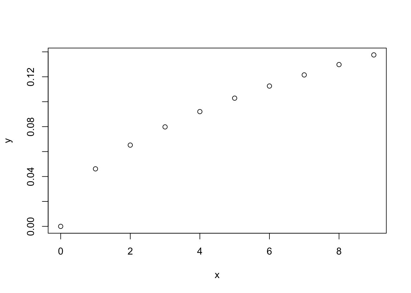

Plot a curve of a function

curve(beta,0,10)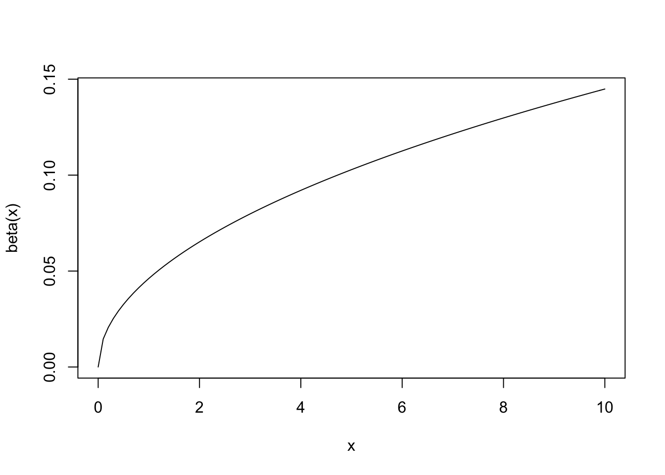

Plot the points, and add a curve to the same plot; also, add some new labels to the axes

plot(x,y,
   xlab="proton kinetic energy [MeV]", ylab="v/c", main="Velocity vs. Kinetic Energy")
curve(beta, 0, 10, add=TRUE, col="blue")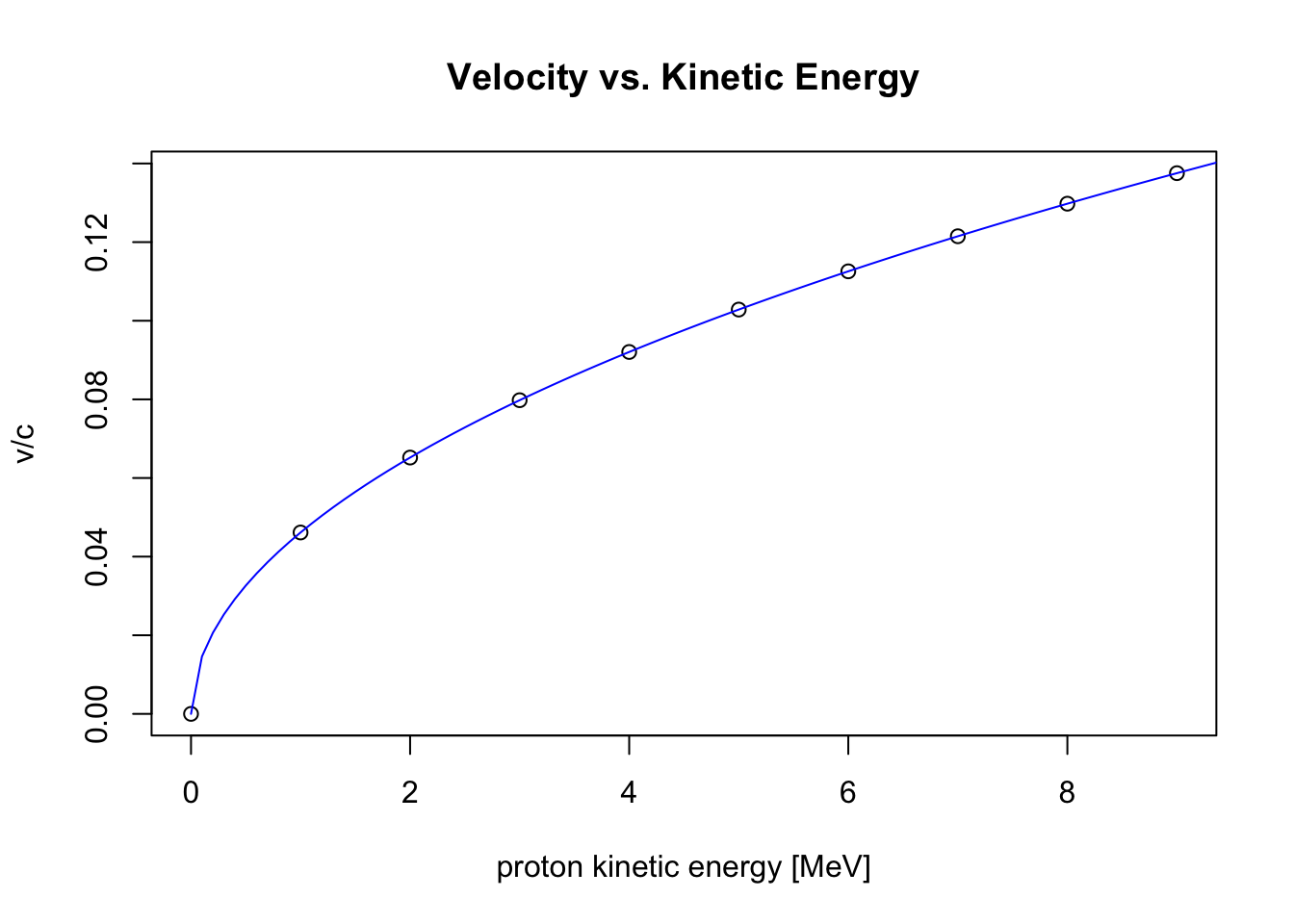

A.3 Creating Random Distributions

# Uniform Distribution of Npts points between 0 and 1
Npts = 500
r = runif(Npts,0,1)
plot(r)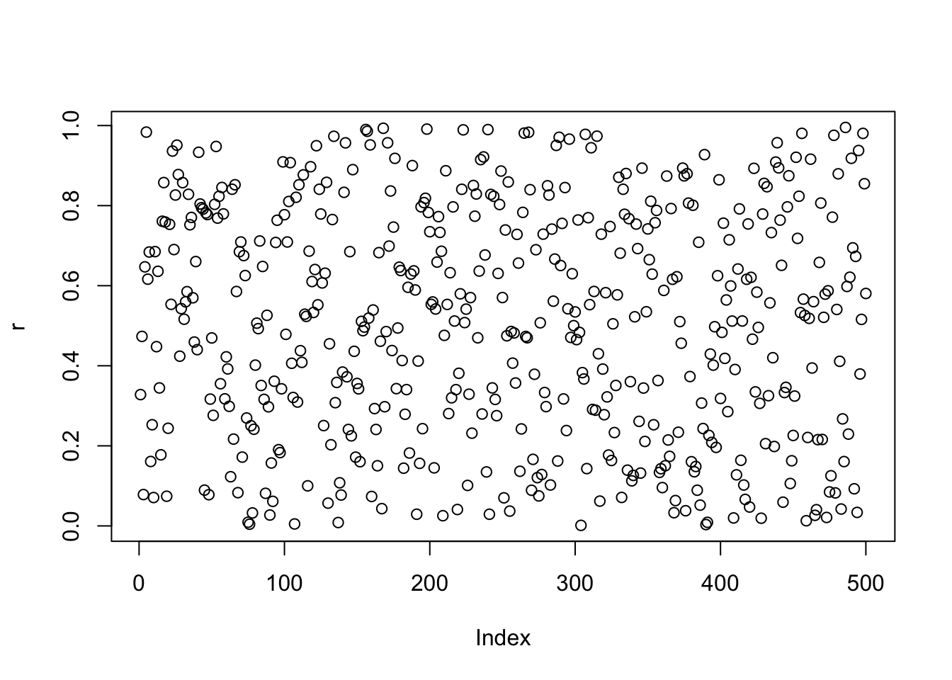

hist(r)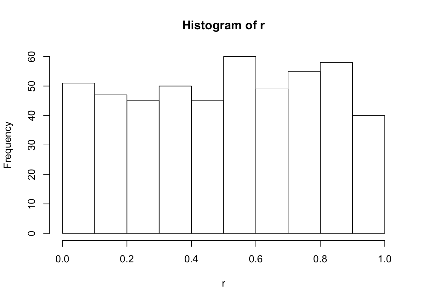

# Normal (Gaussian) Distribution of Npts points, with mean=0, sigma=sig
sig=2
r = rnorm(Npts,0,sig)
plot(r)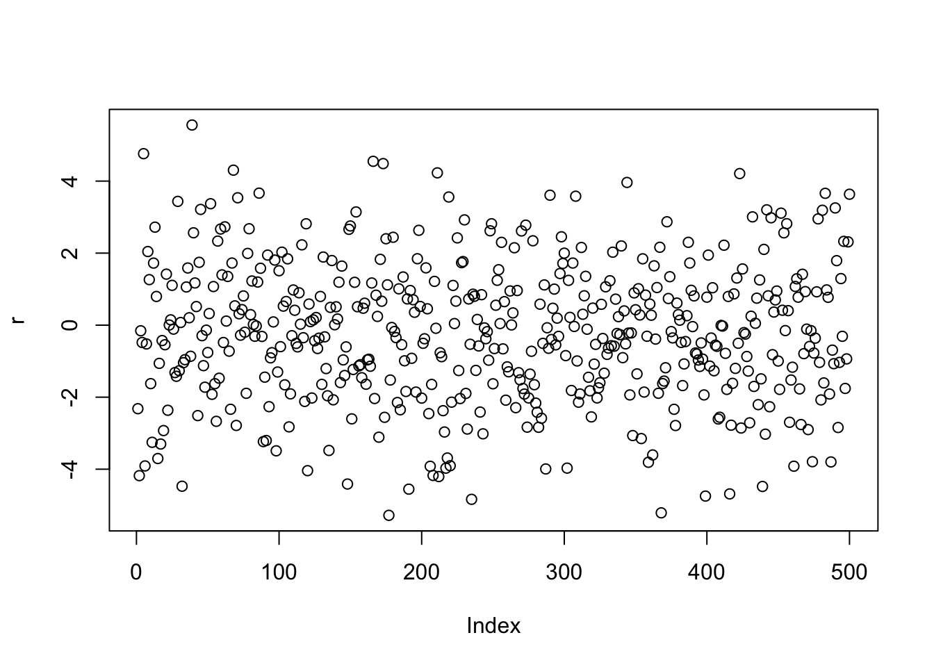

hist(r)
curve(Npts/(sqrt(2*pi)*sig)*exp(-x^2/(2*sig^2)), add=TRUE, col="blue")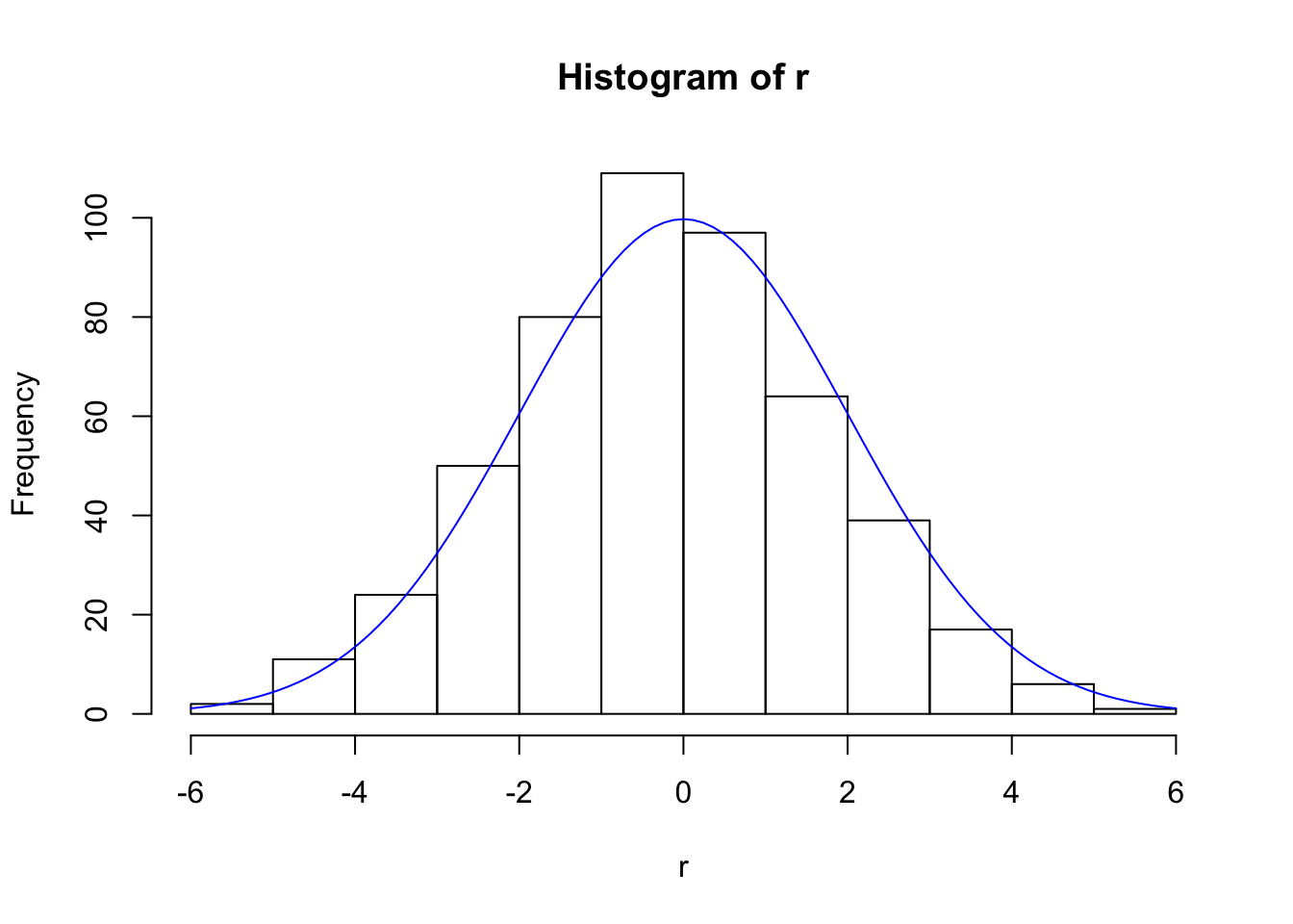

A.4 Decisions and Loops

imax=10
x = array(c(1:imax))
x

##  [1]  1  2  3  4  5  6  7  8  9 10

i = 1
while (i<imax){
  x[i+1] = x[i] + 12
  i = i+1
}
x

##  [1]   1  13  25  37  49  61  73  85  97 109

Can use ifelse(test,yes,no) to perform tests and make decisions

imax=10
x = runif(imax,-1,1)
round(x,2)

##  [1]  0.88 -0.70 -0.60 -0.72 -0.83 -0.91 -0.58 -0.45 -0.54 -0.35

i = 1
while (i<imax+1){
  x[i] = ifelse(x[i]<0, abs(x[i]), x[i])
  i = i+1
}
round(x,2)

##  [1] 0.88 0.70 0.60 0.72 0.83 0.91 0.58 0.45 0.54 0.35

A.5 Matrix Manipulations

A matrix is essentially an ordered list; so, create a list of numbers and tell R where to break the list into rows or columns.

M = matrix( c(1,2,3,4), ncol=2, byrow=TRUE)
M

##      [,1] [,2]
## [1,]    1    2
## [2,]    3    4

Nice to type the input this way, to visually emphasize the arrangement:

A = matrix( c(1, 2,
              3, 4  ), ncol=2, byrow=TRUE)
A

##      [,1] [,2]
## [1,]    1    2
## [2,]    3    4

B = matrix( c(5, 6,
              7, 8  ), ncol=2, byrow=TRUE)
B

##      [,1] [,2]
## [1,]    5    6
## [2,]    7    8

Multiply matrices – but be careful! If you write A * B, this will take each element of A (say a11) and multiply by the corresponding element in B (say b11). What we want is a real matrix multiply – performed using the %*% operator:

C = A * B
C

##      [,1] [,2]
## [1,]    5   12
## [2,]   21   32

WRONG!!

Here’s the right way (in R ):

C = A %*% B
C

##      [,1] [,2]
## [1,]   19   22
## [2,]   43   50

Take the transpose using t(), determinant using det()

t(A)

##      [,1] [,2]
## [1,]    1    3
## [2,]    2    4

det(A)

## [1] -2

To find the inverse of a matrix, we use the solve() function:

solve(A)

##      [,1] [,2]
## [1,] -2.0  1.0
## [2,]  1.5 -0.5

Check:

  A      %*% solve(A)

##      [,1]         [,2]
## [1,]    1 1.110223e-16
## [2,]    0 1.000000e+00

solve(A) %*%   A

##      [,1]         [,2]
## [1,]    1 4.440892e-16
## [2,]    0 1.000000e+00

The function solve(A,B) solves the equation \(A\vec{x} = B\) for \(\vec{x}\). If \(B\) is missing in the solve() command, it is taken to be the identity and the inverse of \(A\) is returned. If you don’t like all the extra digits above, try:

round(solve(A) %*% A, 10)

##      [,1] [,2]
## [1,]    1    0
## [2,]    0    1

Multiply a vector by a matrix to get a new vector; still use the operator %*%…

x = c(2,1)
x

## [1] 2 1

t(t(x))  # trick, to see it in a "usual" (up/down) vector format

##      [,1]
## [1,]    2
## [2,]    1

A

##      [,1] [,2]
## [1,]    1    2
## [2,]    3    4

A %*% x

##      [,1]
## [1,]    4
## [2,]   10

A.6 Reading/Writing Data

Write a set of numbers to a file, and read them back in…

x = rnorm(73,3,6)
y = rnorm(73,0,1)
write(rbind(x,y), file="data.txt", ncol=2)

data = scan("data.txt", list(0,0))
xx = data[[1]]  # first column
yy = data[[2]]  # second column
head(cbind(xx,yy))

##              xx         yy
## [1,] -2.6297200  0.6327915
## [2,] -0.6556138  1.4066700
## [3,] -0.4144076  0.3991774
## [4,] -1.3954840 -0.4804616
## [5,]  6.6422850  1.1156560
## [6,]  2.7988960  0.3387337

plot(xx,yy)
abline(h=mean(yy), v=mean(xx), lty=2)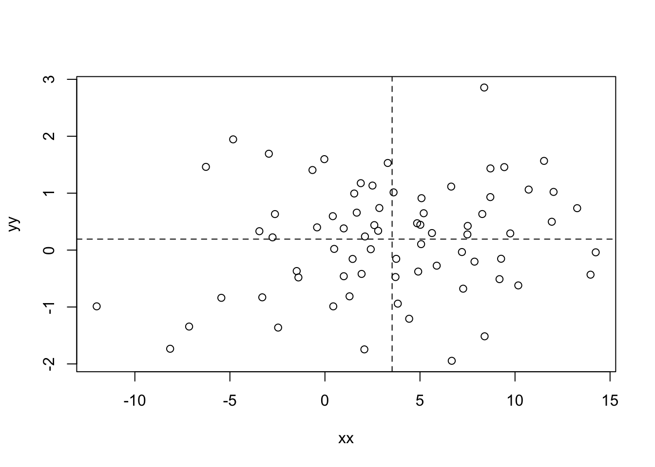

Note: The abline() function adds either horizontal, vertical, or general (\(y = a + bx\)) lines to an existing plot. The argument “lty” determines the type of line (solid, dotted, etc.).

A.7 Dataframes

Often times we wish to create or maybe read in a table of data, perhaps from measurements that were taken or from the results of a computer simulation, and take a quick look at the numbers, make simple plots, or pursue other manipulations. Above we read in data from a file and then identified new variables for each of the two columns of numbers. Below we will generate a new file of data and read it in using the read.table command; this will create a “dataframe” in R which makes many new options available for our use.

# Create some sample data and write to a file, with a header line
x = rnorm(50,0,2)
y = rnorm(50,0,5)
p = (y/5*2-5*x)/10
z = 2-(x+runif(50,-2,2))/2

filename = "data2.txt"
write(c("x","y","z","dp"), file=filename, ncol=4) # creates the file header
write(c(x,y,z,p), file=filename, ncol=4,append=TRUE) # writes the data

Next, we read the file back in, creating a dataframe named “data”.

filename = "data2.txt"
data = read.table(file=filename,header=TRUE,sep="")
# What have we created?
attributes(data)

## $names
## [1] "x"  "y"  "z"  "dp"
## 
## $class
## [1] "data.frame"
## 
## $row.names
##  [1]  1  2  3  4  5  6  7  8  9 10 11 12 13 14 15 16 17 18 19 20 21 22 23
## [24] 24 25 26 27 28 29 30 31 32 33 34 35 36 37 38 39 40 41 42 43 44 45 46
## [47] 47 48 49 50

head(data)  # look at first few lines of the dataframe

##            x         y          z         dp
## 1 -0.2745031  1.470061 -0.7219688  0.4497794
## 2 -0.2181247 -3.968991 -1.4216170 -0.6302756
## 3  2.0312670  2.970257  0.6366110 -0.9012050
## 4  3.0867700 -4.408427  1.0105010 -0.6646915
## 5 -1.4574350  5.432393 -2.6866640 -0.9475328
## 6 -2.0257210 -1.333614  4.8103560 -1.1374940

Note that the names of the columns in our dataframe are taken from the header (first line) of the text file we read in. To access the data for one of the variables (columns) from our dataframe data we use the dollar sign:

length(data$x) # number of entries for "x"

## [1] 50

data$x[23]     # value of 23rd entry for "x"

## [1] -0.2883335

print(sqrt(abs(data$x)))  # perform calculation on all values of "x"

##  [1] 0.5239304 0.4670382 1.4252252 1.7569206 1.2072427 1.4232783 0.6163714
##  [8] 1.0796597 1.4363523 1.3737962 1.4855167 0.3572415 0.3491438 1.0557575
## [15] 0.7532369 1.1989337 0.5686237 2.6971778 1.8356487 1.8859557 2.7977906
## [22] 2.6267794 0.5369669 2.3024083 1.1156411 1.6831257 1.5163934 1.3663510
## [29] 0.7779226 1.5983517 1.7439163 1.1370295 1.7245130 1.4781766 0.7950262
## [36] 1.8368615 1.2384599 1.1678365 0.5624940 0.8564480 0.6130279 0.7016532
## [43] 1.0258367 1.5067827 0.9994675 1.6374202 1.3281739 0.9759249 0.6963378
## [50] 0.5119257

pairs(data)    # create plots of each varialble vs. every other variable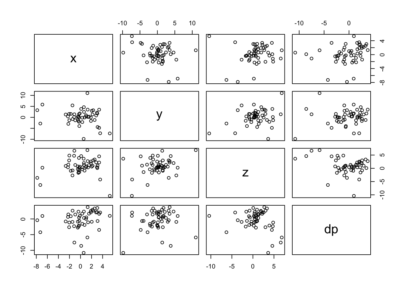

plot(data$x,data$dp)  # plot one variable vs. another variable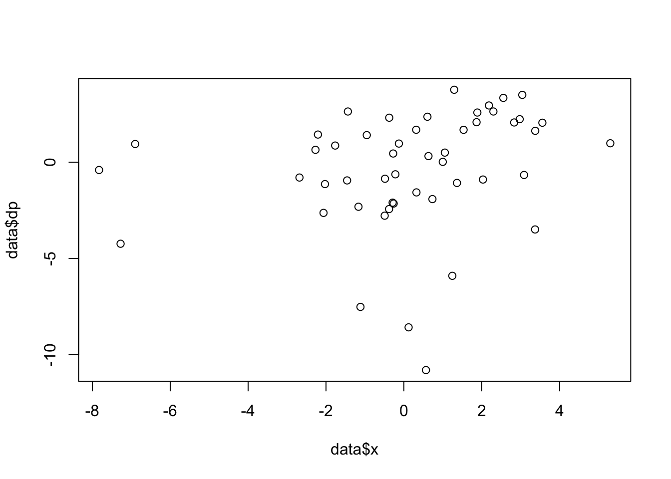

You can create a subsest of your dataset:

# find subset where abs(x)<0.8 AND abs(y)<1:
data_sub = subset(data, subset=( (abs(data$x)<4) & (abs(data$y)<1)) )
length(data_sub$x)

## [1] 14

plot(data_sub$x,data_sub$dp)  # plot one variable vs. another variable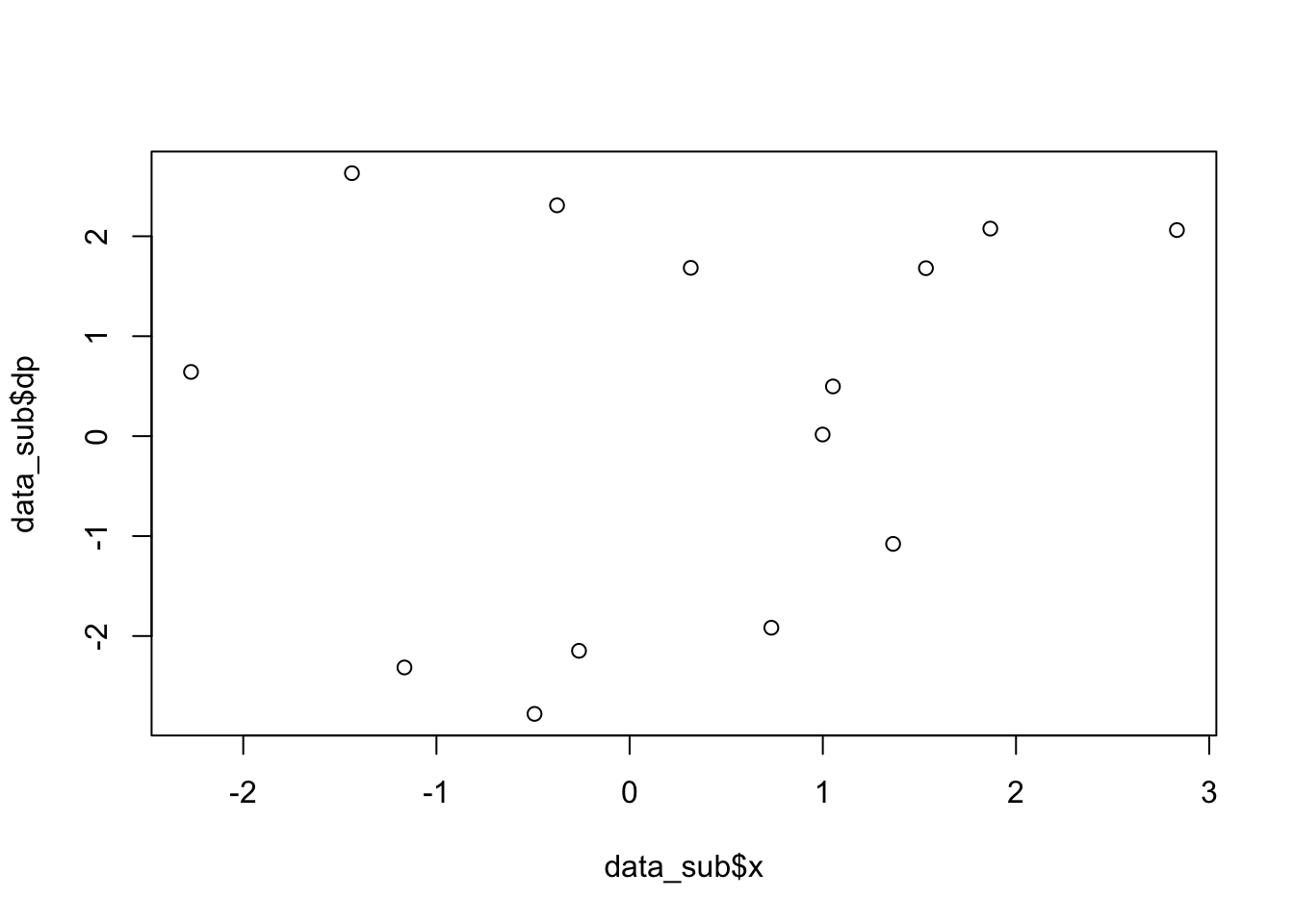

#  note: a & b     "a is true AND b is true" (intersection)
#        a | b     "a is true OR  b is true"    (union)
#         !a            "a is NOT true"        (negation)
#      other logical options:  a< b  a<=b  a==b  a>=b   a!=b   

Next, we take our plot and fit the data to a linear model, finding the intercept and slope, and adding the corresponding line to the plot

fitparams = lm(dp ~ x, data_sub)
fitparams

## 
## Call:
## lm(formula = dp ~ x, data = data_sub)
## 
## Coefficients:
## (Intercept)            x  
##      0.1383       0.3041

plot(data_sub$x,data_sub$dp)
abline(a=fitparams$coef[1], b=fitparams$coef[2],lty=2,col="red")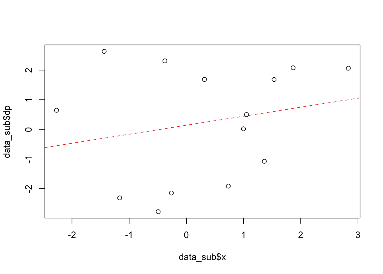

A.8 Connecting to External Programs

It is sometimes desired to run other outside software packages from inside R, for example to create data files that can then be read in. To do so, one can use the system() function. As an example, suppose we want to execute the program MAD-X with an input file named input.madx:

on PC:

system(“cmd.exe”, input=“madx input.madx”)

on Mac/Linux:

system(“./madx input.madx”)

Before executing the program, one may need to change the working directory to that of the program itself. Do so using

setwd(“path/to/program”)

where path/to/program uses the correct path syntax of the operating system being used.

A.9 And Much, Much … Much, Much More

text manipulations; complex plotting control; optimizations; complex statistical analyses and modeling; …

visit: https://www.r-project.org/ for more information