Final Topics
Friday Morning Class Presentations
Two or Three Teams of 2-3 students:
Each team choose one topic below to address and present for Friday morning. Present your results/findings to the group in the style of a 20-minute talk at a conference or APS meeting. Allow 10 minutes for discussion (i.e., grilling by the instructors).
Wedge Cooling. Discuss the desire and purpose of a wedge for altering the momentum distribution of the muon beam for \(g\)-2. In particular,
For a particle at 3160 MeV/c, determine the Beryllium (Be) thickness needed to reduce its momentum to 3100 MeV/c (magic). Repeat the same for Nickel (Ni).
Estimate the width of the Coulomb multiple scattering angle for both materials. Comment on your results.
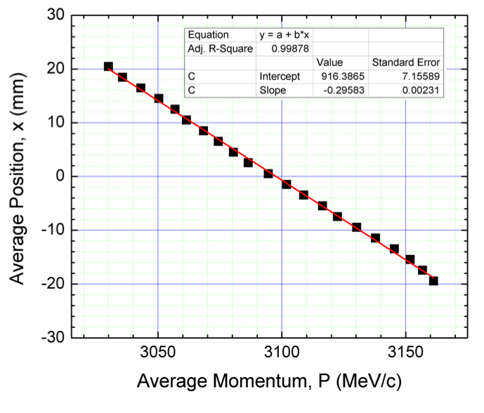
Assume that you have a beam passing through a dispersive area so that a strong correlation between momentum and horizontal position builds up. Suppose that the position of each particle varies linearly with momentum as shown in the plot below. For particles with P>3100 MeV/c but P<3165 MeV/c, make a plot of the required material thickness to cool to 3100 MeV/c vs momentum (take 10-15 points). Do so for both Be and Ni. Comment on your results.
Indirectly, you have constructed a wedge. For a Be and Ni wedge, what its height, angle and base?
 \(\hspace{0.1in}\)
Final Momentum. We wish to maximize the intensity of the stored muon beam, but would also like to have as small a momentum spread as possible. Assuming a constant initial distribution entering the ring from the beam delivery system, explore options of round apertures, square apertures, or other configurations that might address these concerns, and report on your findings.
Frozen Spins. Explain to the audience the ways in which one would wish to design a storage ring to search for/measure an electric dipole moment (EDM) signal using a polarized beam. Consider, for instance, a storage ring in which a particle’s ideal circular orbit is created using a uniform vertical magnetic field of magnitude \(B_0\) as well as a radial electric field of magnitude \(E_0\) along the design orbit.
Assuming that a positive value of \(B_0\) is in the positive vertical direction and a positive value of \(E_0\) is directed radially inward, show that the “frozen spin” condition, where \(\omega_a = 0\), is met when \[ E_0 = \frac{a\beta\gamma^2}{1-a\beta^2\gamma^2}\cdot B_0c. \]
Suppose we use an electric field of 10 MV/m and a magnetic field of 1.8 T to create a frozen spin condition for a positive muon. What would its momentum need to be?
With \(\omega_a = 0\) established, what signal would one expect to see for a particle with a non-zero EDM?
What sources of systematic error will be important in this measurement and how might they be addressed?
Flight for Survial. Consider particles that are undergoing betatron oscillations – both horizontally and vertically – that have amplitudes capable of consipring to reach the physical aperture (\(a_0\) = 45 mm). Ultimately we would like to know the average rate at which particles will reach within 0.5 mm of the aperture, at which point we can assume that they will likely be lost. Possible questions to answer:
- What is the average number of turns that such a particle can survive before coming within 0.5 mm of the aperture?
- How does this lifetime and/or loss rate depend upon the choice of tunes (quadrupole voltage setting)?
- Is there a correlation between number of turns survived (as defined in part (a)) and particle momentum \(\Delta p/p\)?
- What is the average number of turns that such a particle can survive before coming within 0.5 mm of the aperture?
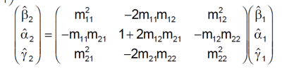
Quad Scan Emittance Measurement. Suppose that you have a beamline that contains a quadrupole magnet of length \(L\) (\(L\) = 609.60 mm) and a downstream drift of length, \(d\) (\(d\) = 11155.78 mm). Suppose that the Twiss parameters at the entrance to quad are \(\alpha_1\), \(\beta_1\), \(\gamma_1\) (Position 1) and downstream at the end of the drift are \(\alpha_2\), \(\beta_2\), \(\gamma_2\) (Position 2). Assume that the emittance is conserved along the beamline.
If \(m_{11}\), \(m_{12}\), \(m_{21}\), \(m_{22}\), are the elements of the transport matrix \(M\) between Position 1 and Position 2, show that the Twiss parameters between these two points transform according to:
 \(\hspace{0.1in}\)
Suppose that you have placed a profile monitor at Position 2 wherein you record the beam size versus quad focusing strength, \(\kappa\). All data are contained in the table below. Note that the first column is \(\kappa\) in m\(^{-2}\), the second column is the \(x\)-rms-size in mm and the third column is the \(y\)-rms-size in mm. By applying the quad-scan technique discussed in class, estimate the beam rms emittance and Twiss parameters in Position 1 in both \(x\) and \(y\) planes. Hint: Plot the rms beam size squared vs. magnet strength first. Then, do a (non-linear) fit of the data to the theoretical expression (between rms squared and focusing strength) derived from the expression in question (a). You may have to use MATLAB or Mathematica or an equivalent program to do the fit.
Repeat the same but this time using a thin lens approximation (\(L\rightarrow 0\)). This implies that the Twiss parameters are calculated at the center of the lens. Hint: The center of the thin lens should be at the center of the full-length quad, hence you may have to alter the drift sections upstream and downstream of the thin lens. Another Hint: You may end up in a parabolic expression between rms beam size squared and magnet strength, as we discussed in class.
Compare your answers in (b) and (c) and discuss the results. Hint: Make sure that the comparison is done at the same \(z\)-location.
| \(\kappa\) (m\(^{-2}\)) | \(\sigma_x\) (mm) | \(\sigma_y\) (mm) |
|---|---|---|
| 0.100304 | 23.68029 | 17.04768 |
| 0.13265 | 21.55388 | 16.64572 |
| 0.164997 | 19.48502 | 16.31624 |
| 0.197344 | 17.23853 | 16.08798 |
| 0.213517 | 16.14946 | 16.03975 |
| 0.229691 | 15.04892 | 15.98315 |
| 0.245864 | 13.97309 | 15.95849 |
| 0.262038 | 12.9633 | 15.96675 |
| 0.278211 | 11.96482 | 15.99507 |
| 0.294384 | 11.03464 | 16.05166 |
| 0.310558 | 10.20846 | 16.14522 |
| 0.326731 | 9.469429 | 16.25822 |
| 0.342905 | 8.86313 | 16.39863 |
| 0.359078 | 8.417069 | 16.56607 |
| 0.375251 | 8.157031 | 16.75962 |
| 0.391425 | 8.099382 | 16.97878 |
| 0.407598 | 8.247382 | 17.22273 |
| 0.423772 | 8.58909 | 17.49038 |
| 0.439945 | 9.101957 | 17.78116 |
| 0.456118 | 9.757619 | 18.09362 |
| 0.472292 | 10.52852 | 18.4271 |
| 0.488465 | 11.39107 | 18.78084 |
| 0.504639 | 12.3243 | 19.15344 |
| 0.520812 | 13.31301 | 19.54417 |
| 0.536985 | 14.34578 | 19.95219 |
| 0.553159 | 15.3822 | 20.34611 |