D Creation and Analysis of Beam Distributions
Codes like g4beamline, COSY, BMAD, etc., have tracking algorithms for transporting particles from one point to another and can generate beam distributions along a beam line. Often times one wants to express these distributions in terms of their areas in phase space (emittance) and their shape and orientation (Courant-Snyder parameters) in phase space as well as their dispersive characteristics with respect to momentum (dispersion). On the other hand, sometimes one has a beam line design with Courant-Snyder parameters and dispersion provided to the user and one would like to generate a “matched” distribution of particles to track through the beam line. Below we discuss techniques to create desired distributions from given optics parameters or to analyze given distributions to determine the optics parameters describing them.
The concepts of phase space ellipses, Courant-Snyder parameters (sometimes called Twiss parameters) and lowest-order dispersion come from linear, uncoupled theory. There are ways to describe linearly coupled motion with similar notation, though this is much more complicated. In practice, beam line designers typically attempt to minimize the coupling between the two transverse degrees of freedom as much as possible, and hence, to the degree that this is true, one can talk about Courant-Snyder parameters (\(\beta\), \(\alpha\)), dispersion (\(D\)) and emittance (\(\epsilon\)) as having separate sets of values for the vertical motion and for the horizontal motion. We assume this is the case for the following arguments.
Let’s assume that in the absence of dispersion (i.e., all particles are following the same central trajectory, independent of momentum) that a particle’s motion is given by transverse coordinate \(x_\beta\) due to betatron oscillations about the ideal trajectory. In terms of Courant-Snyder variables and emittance, if we average over the ensemble of particles we would define
\[\begin{eqnarray*} \langle x_\beta^2 \rangle &=& ~\epsilon\beta \\ \langle x_\beta'^2 \rangle &=& ~\epsilon\gamma \\ \langle x_\beta x_\beta'\rangle &=& -\epsilon\alpha \end{eqnarray*}\]and the relationship between the three Courant-Snyder parameters is \[ \beta\gamma-\alpha^2 = 1. \] In the above, the particle distribution is assumed to be centered about the ideal trajectory.
Now suppose, after passing through bending elements, the trajectories of the various particles become dispersed by the amount \(D\delta\), where \(D\) is the dispersion function and \(\delta = \Delta p/p\) is the relative momentum deviation of an individual particle. Along our central design trajectory the total displacement \(x\) of a particle would be \[ x = x_\beta + D\delta. \] We use the above to find the following averages taken over the distribution of our particle ensemble:
\[\begin{eqnarray*} \langle x^2 \rangle &=& \langle x_\beta^2\rangle + \langle x_\beta\;D\delta\rangle +\langle D^2\delta^2\rangle = \epsilon\beta + D^2\langle\delta^2\rangle \\ \langle x'^2\rangle &=& \epsilon\gamma + D'^2\langle\delta^2\rangle \\ \langle x'x\rangle &=& -\epsilon\alpha + D'D\langle\delta^2\rangle \\ \langle x\cdot\delta\rangle &=& \langle x_\beta\delta\rangle + \langle D\delta^2\rangle = D\langle\delta^2\rangle \\ \langle x'\cdot\delta\rangle &=& \langle x_\beta'\delta\rangle + \langle D'\delta^2\rangle = D'\langle\delta^2\rangle \end{eqnarray*}\]Thus we can take our tracking data in which values of \(x\), \(x'\) and \(\delta\) for each particle have been computed (and likewise for the vertical coordinates) and find the values of the dispersion function, Courant-Snyder parameters and emittance that describe the distribution. We obtain:
\[\begin{eqnarray*} D &=& \frac{\langle x\;\delta\rangle}{\langle\delta^2\rangle} \\ D' &=& \frac{\langle x'\;\delta\rangle}{\langle\delta^2\rangle} \\ \epsilon\beta &=& \langle x^2\rangle - \frac{\langle x\;\delta\rangle^2}{\langle\delta^2\rangle} \\ \epsilon\gamma &=& \langle x'^2\rangle - \frac{\langle x'\;\delta\rangle^2}{\langle\delta^2\rangle} \\ \epsilon\alpha &=& -\langle xx'\rangle + \frac{\langle x'\;\delta\rangle\langle x\;\delta\rangle}{\langle\delta^2\rangle} \\ \epsilon &=& \sqrt{(\epsilon\beta)(\epsilon\gamma)-(\epsilon\alpha)^2} \end{eqnarray*}\]and hence \(\epsilon\), \(\beta\), \(\alpha\), \(D\) and \(D'\) can all be computed from the particle distribution in \(x,x'\), and likewise for \(y,y'\).
Creating a Distribution
As a concrete example, let’s create a distribution of particles for a given set of parameters, then use our equations above to analyze the distribution to verify that we get the original parameters back.
Suppose we have the following target values for Courant-Snyder variables and dispersion of our beam distribution:
beta = 17.0     # m
alf  = -2.5
emit = 12.0     # pi mm-mr
D    =  1.4     # m
Dp   =  0.015
We will assume that our phase space variables, including momentum deviation, are distributed normally (Gaussian). To generate the distribution, we note that the phase space trajectories in \(x\) - \((\beta x' + \alpha x)\) phase space are circular; thus we first generate a circular distribution in two variables, using the rms value obtained by the given emittance and value of \(\beta\):
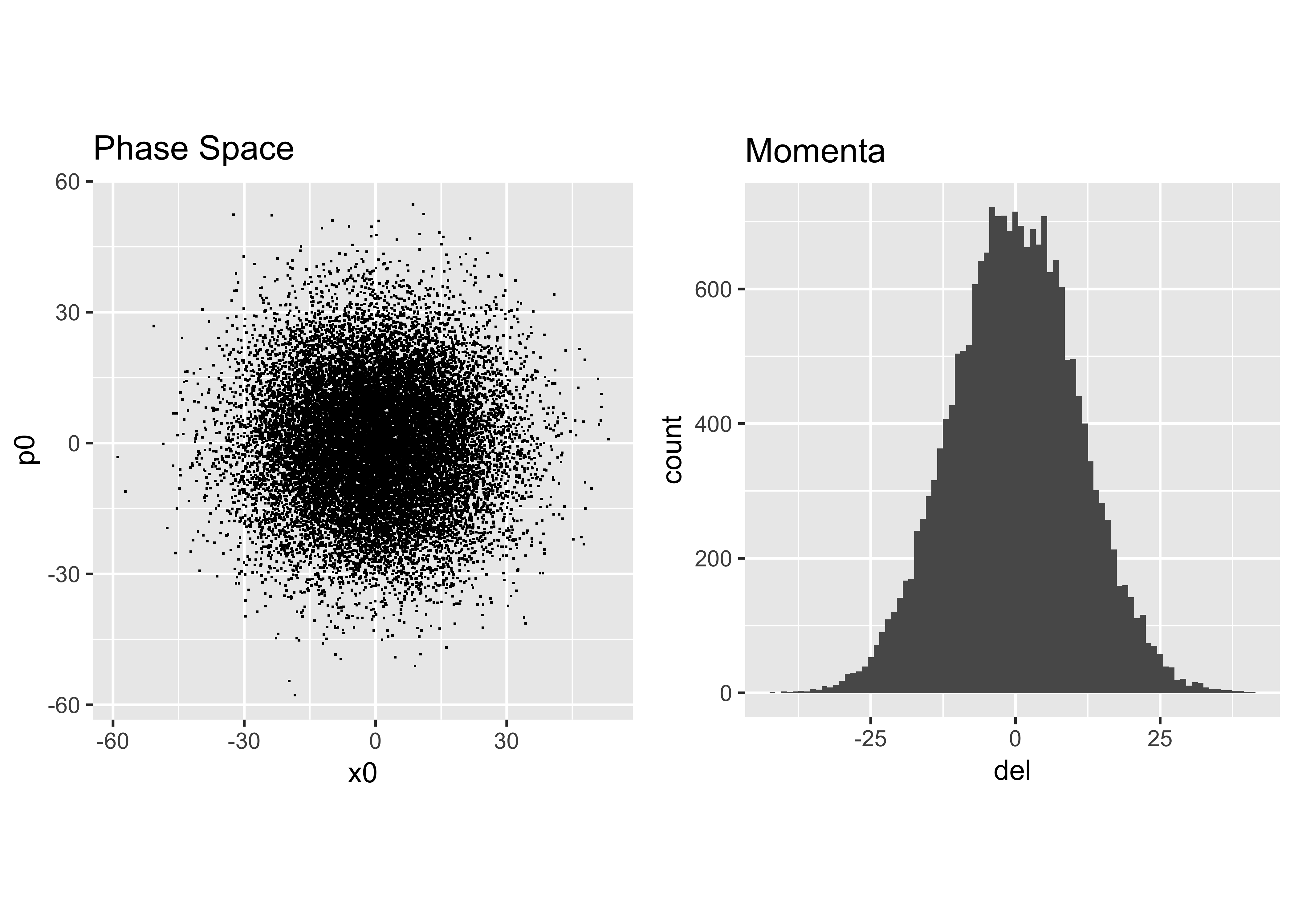
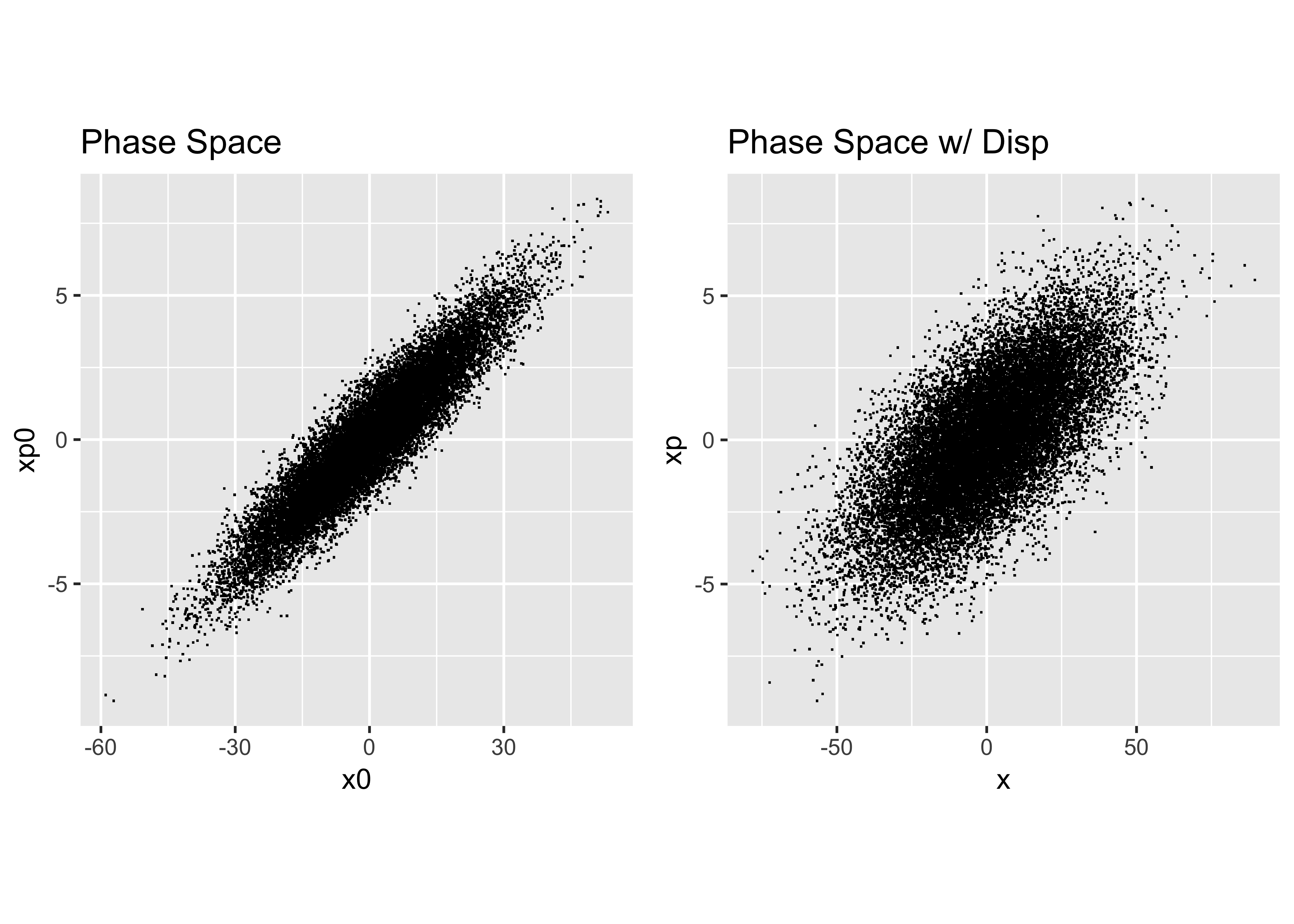
Np   = 20000
sigx =  sqrt(beta*emit)
x0    = rnorm(Np,0,1)*sigx
p0    = rnorm(Np,0,1)*sigx
From the above we can then find the slope \(x'\) of each particle using
xp0 = (p0-alf*x0)/betaNext, we include the momentum distribution and the effects of dispersion. If the rms of the relative momentum deviation distribution is expressed in units of \(10^{-3}\) and the dispersion function in meters, then the result is given inm mm. Thus, the final coordinates will be:
sigp = 11.0                # e-3
del  = rnorm(Np,0,1)*sigp  # e-3
x    = x0  +  D*del        # mm
xp   = xp0 + Dp*del        # mr
p    = alf*x+beta*xp       # mm
Here is our final result:
Analyze the Distribution
Next we take the distribution we just created and perform our earlier analysis to obtain the Courant-Snyder parameters and dispersion that describe it:
Axx   = sd(  x)^2
Axpxp = sd( xp)^2
Add   = sd(del)^2
Axxp  = mean((x-mean(x))*(xp-mean(xp)))
Axd   = mean((x-mean(x))*(del-mean(del)))
Axpd  = mean((xp-mean(xp))*(del-mean(del)))


DF    =  Axd /Add
DpF   =  Axpd/Add
ebetF =  Axx   -    Axd^2/Add
egamF =  Axpxp -   Axpd^2/Add
ealfF = -Axxp  + Axpd*Axd/Add
emitF = sqrt(ebetF*egamF-ealfF^2)

betaF = ebetF/emitF
alfF  = ealfF/emitF
Compare with original parameters:
| Parameter | Original | Analysis | Unit | rel. dev. (%) |
|---|---|---|---|---|
| \(\beta\) | 17 | 16.904 | m | -0.57 |
| \(\alpha\) | -2.5 | -2.483 | -0.67 | |
| \(\epsilon\) | 12 | 11.992 | mm-mr | -0.06 |
| \(D\) | 1.4 | 1.394 | m | -0.45 |
| \(D'\) | 0.015 | 0.014 | -9.04 |
D.1 Normal vs. Uniform Distributions
The code snippets above create Gaussian distributions, but sometimes one wants a uniform distribution in phase space. The following code chunks give simple examples:
x = runif(2000,-1,1)  # uniform between x = (-1,1)
p = runif(2000,-1,1)  # uniform between p = (-1,1)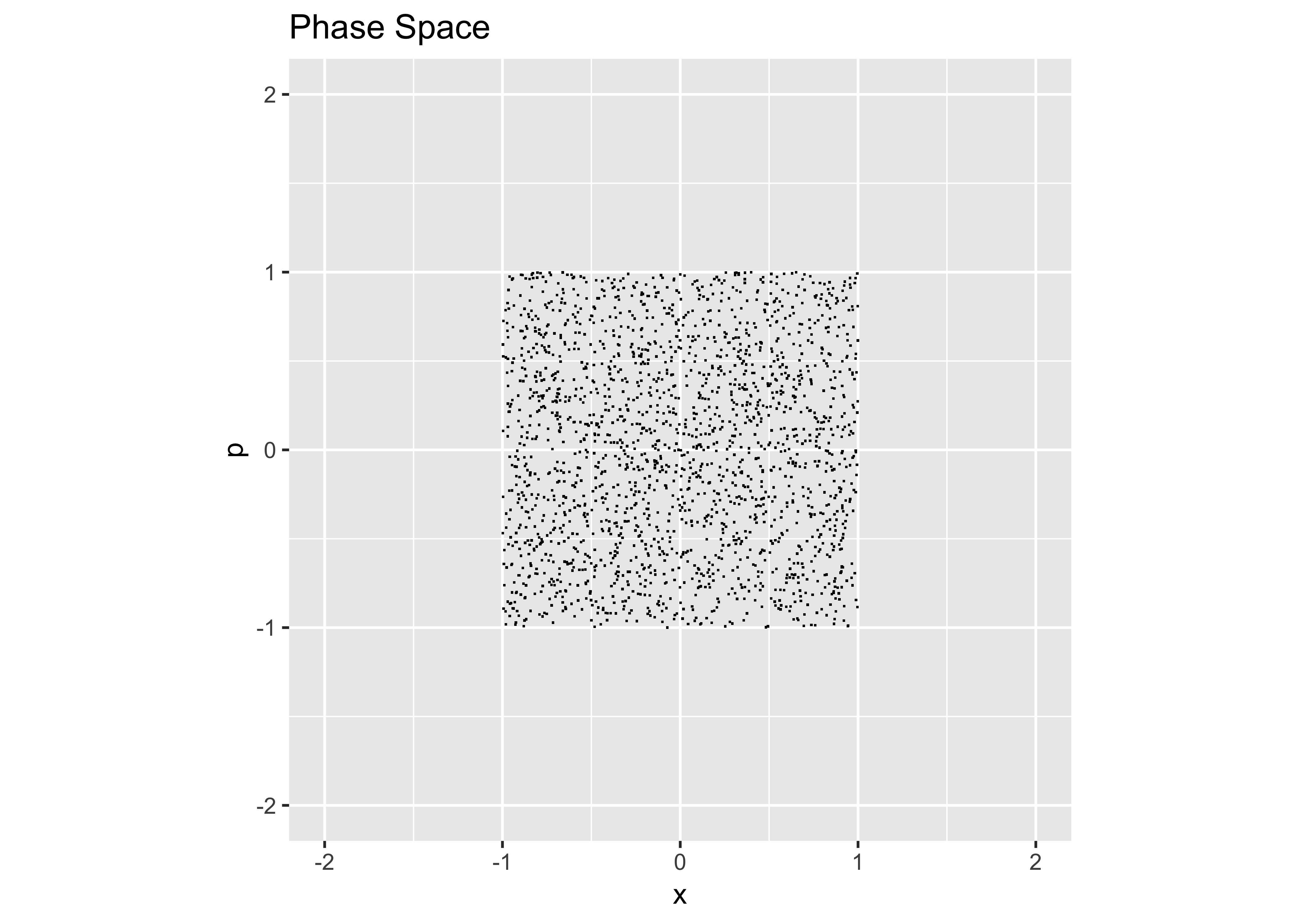
However, to make a round, uniform distribution,…
theta = runif(2000,0,2*pi)    # uniform angle
r = sqrt(runif(2000,0,1))*7   # range of radii, out to r=7
x = r*cos(theta)
p = r*sin(theta)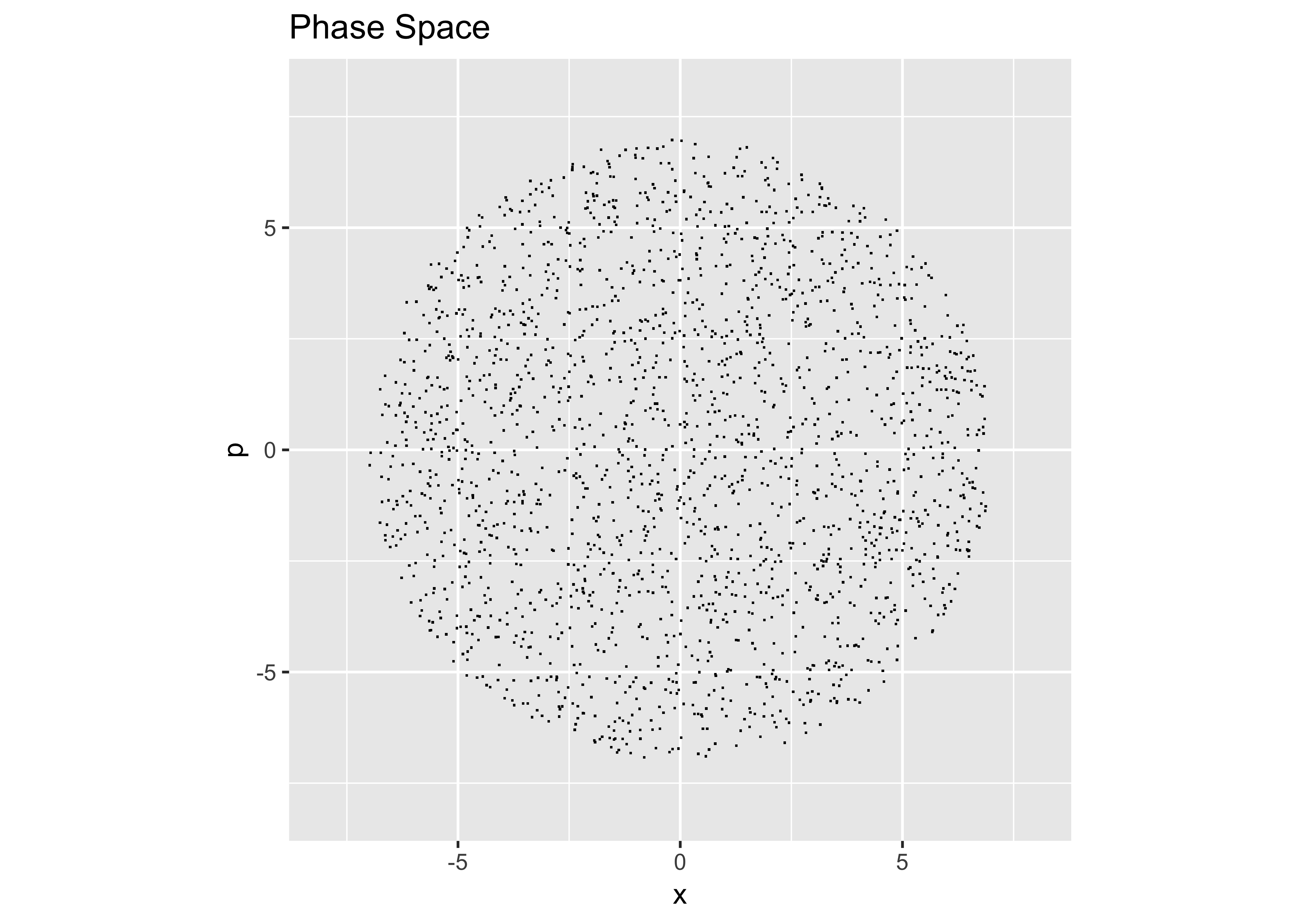
If a Gaussian distribution is desired but access only to a uniform random number generator is available, try the following:
Np = 5000
sig = 5
a1 = runif(Np,0,1)
a2 = runif(Np,0,1)
x = sig*sqrt(-2*log(a1))*(cos(2*pi*a2))
p = sig*sqrt(-2*log(a1))*(sin(2*pi*a2))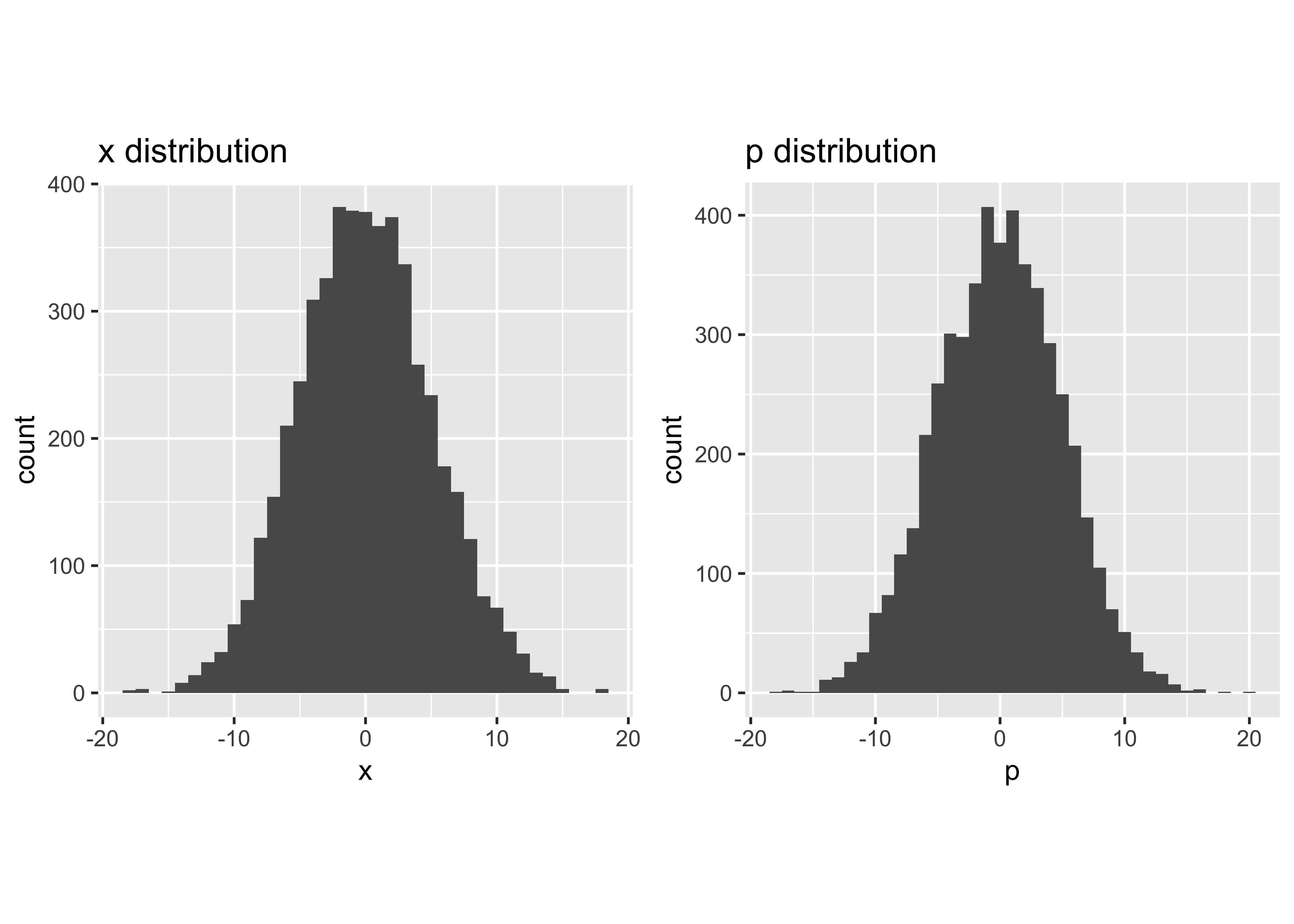
D.2 Creating Distributions from Arbitrary Curves
Sometimes one is given a probability density curve and a sample of particles representing that distribution is desired. An example might be a set of particles distributed in time that mimics a measured beam current pulse from a detector.
Example 1: Create a distribution from a given functional form.
For instance,
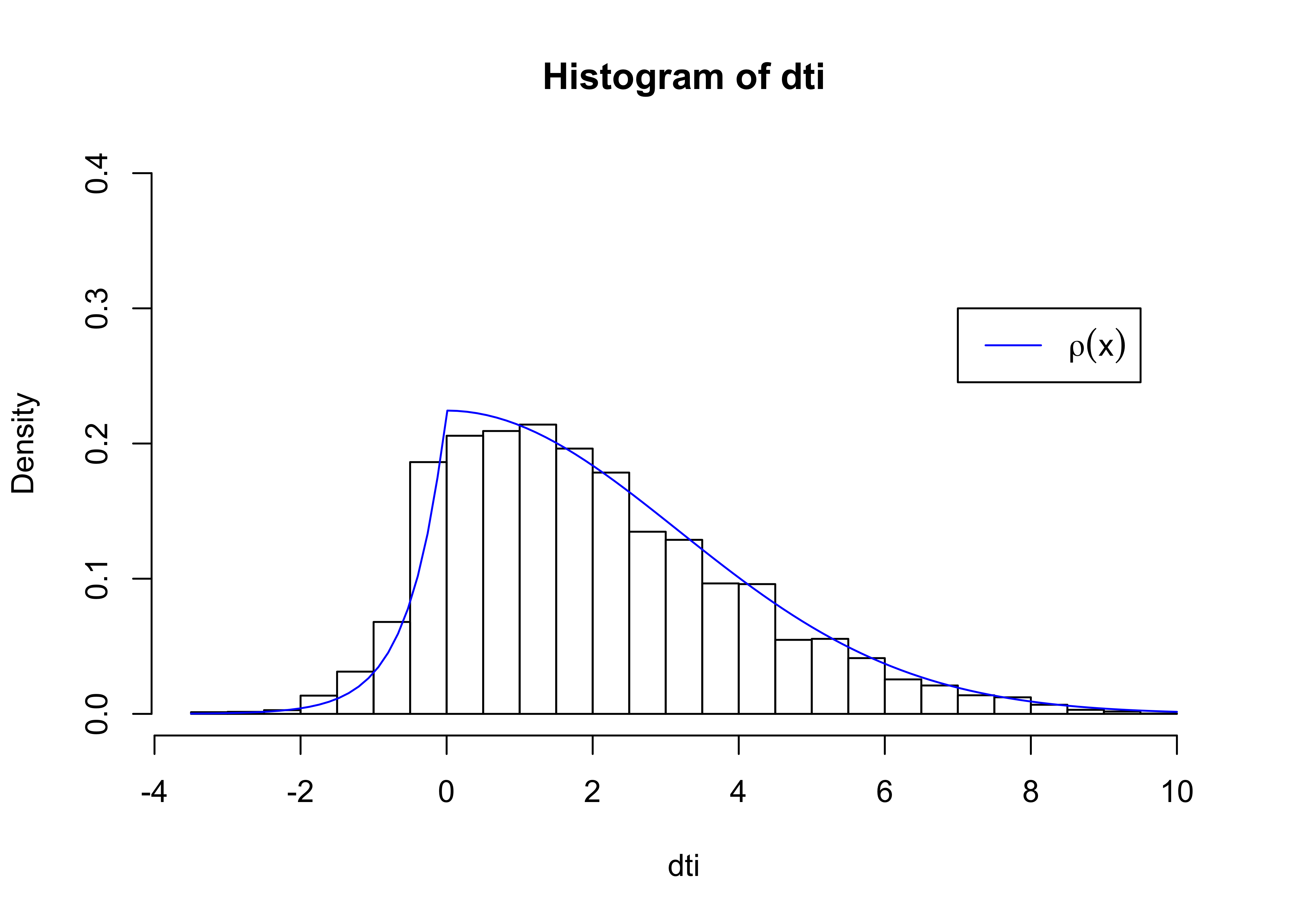
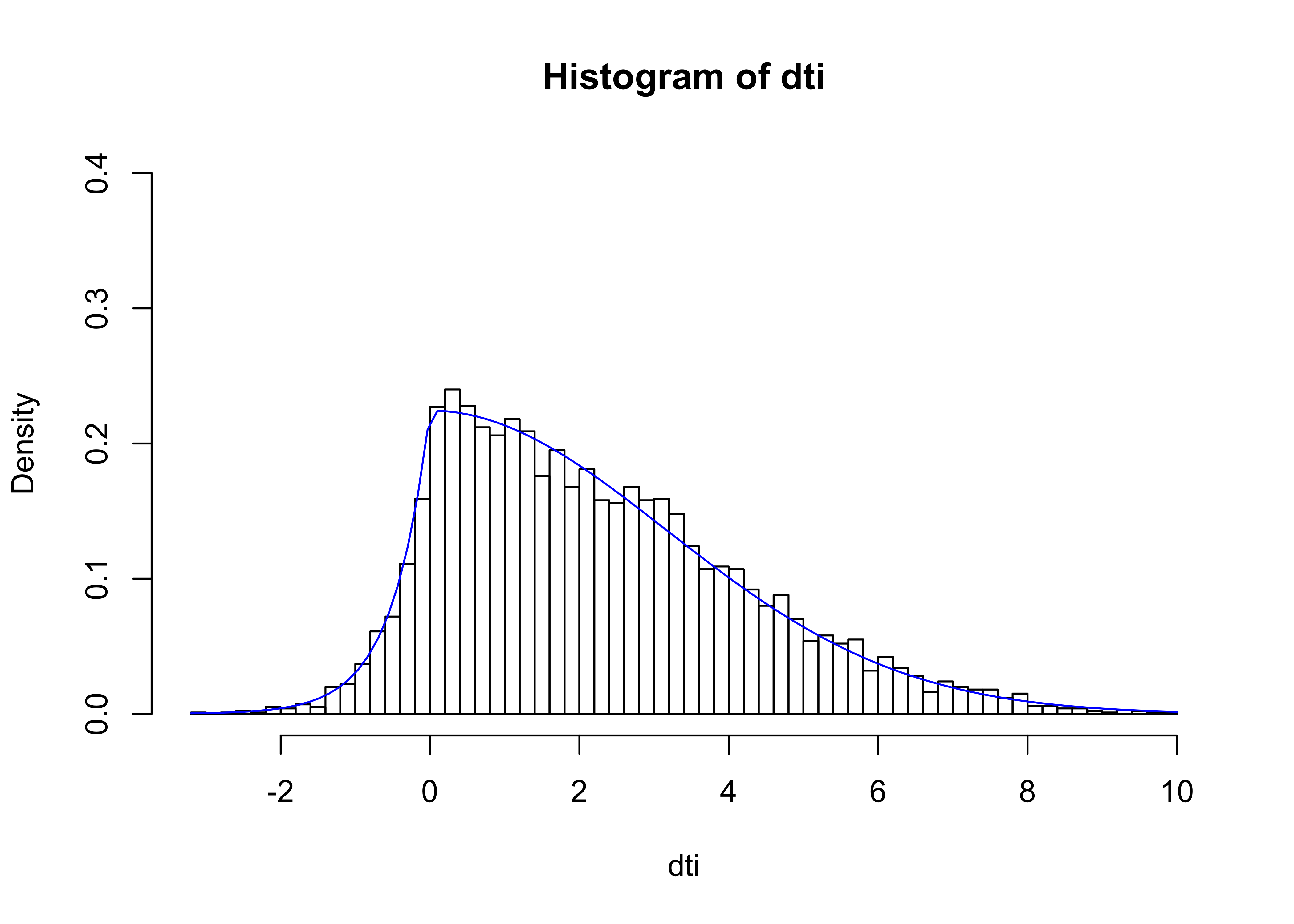
rho0 = function(x){ ifelse(x<0, exp(2*x),exp(-x^2/20)) }
rhoA = integrate(rho0,-4,10)$val
rho = function(x) { rho0(x)/rhoA}    # normalized, integrates to 1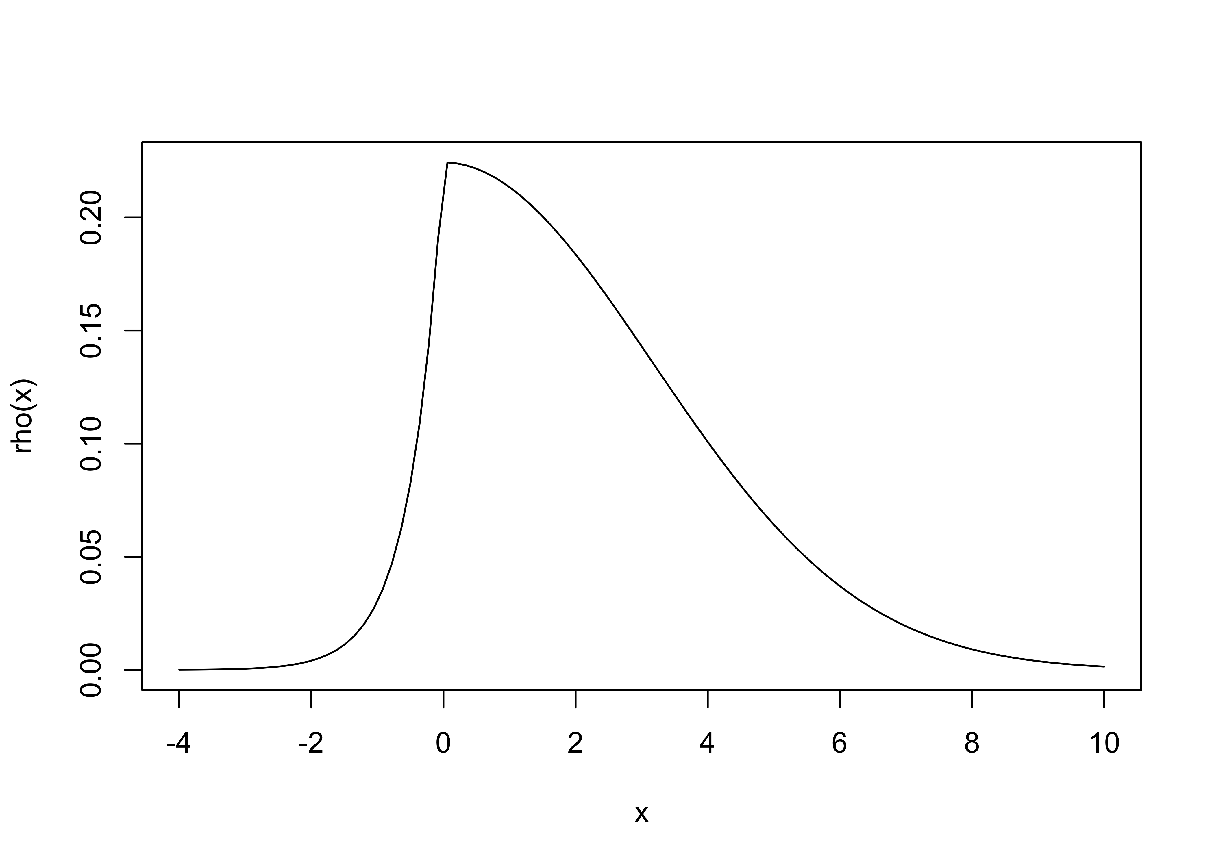
Given our distribution function \(\rho\) above we next create a new function that is the integral of \(\rho\) and hence provides us with the cumulative density function: \(\text{cdf}(x) = \int_0^x \rho(x)dx\)
cdf = function(z) { integrate(rho,-4,z)$val }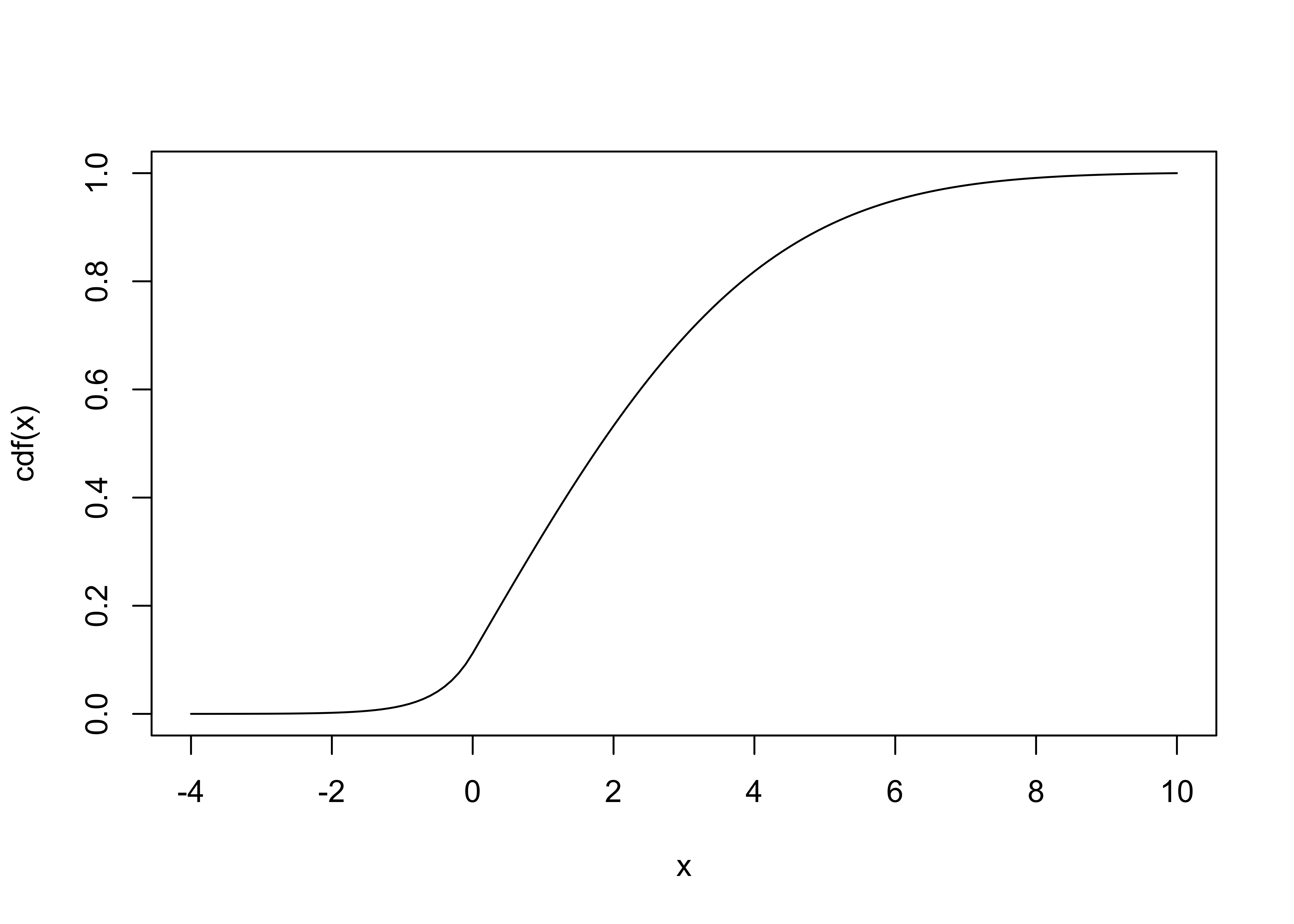
Next we need another new function that we will use to find the inverse of \(cdf(x)\) given a value \(y = \text{cdf}(x)\): \(x = \text{cdf}^{-1}(y)\).
cdfInv = function(y){
   opInv  = function(x){abs(cdf(x)-y)}
   xout = optimize(opInv,c(-4,10))
   as.numeric(xout$minimum)
}
Since the range of the cumulative distribution function is from 0 to 1, we can take a collection of uniformly distributed random variables over the same range and solve for the value of \(x\) that contributes to that value of the cumulative density function.
dtst = runif(Np,0,1)
dti = c(1:Np)*0                  # vector of initial dt of the particles
i = 0
while(i<Np){
   i = i+1
   dti[i] = cdfInv(dtst[i])
}
Plotting a histogram our results, we see that the distribution we generated of the variable dti nicely mimics our desired curve.
Example 2: Create a distribution from a measured curve.
Suppose instead of knowing the exact functional form of the distribution we instead have a discrete measurement or set of ordered pairs of data that represents our desired distribution. For instance, rather than having the curve above, suppose we have a set of points that, perhaps, were obtained through a measurement:
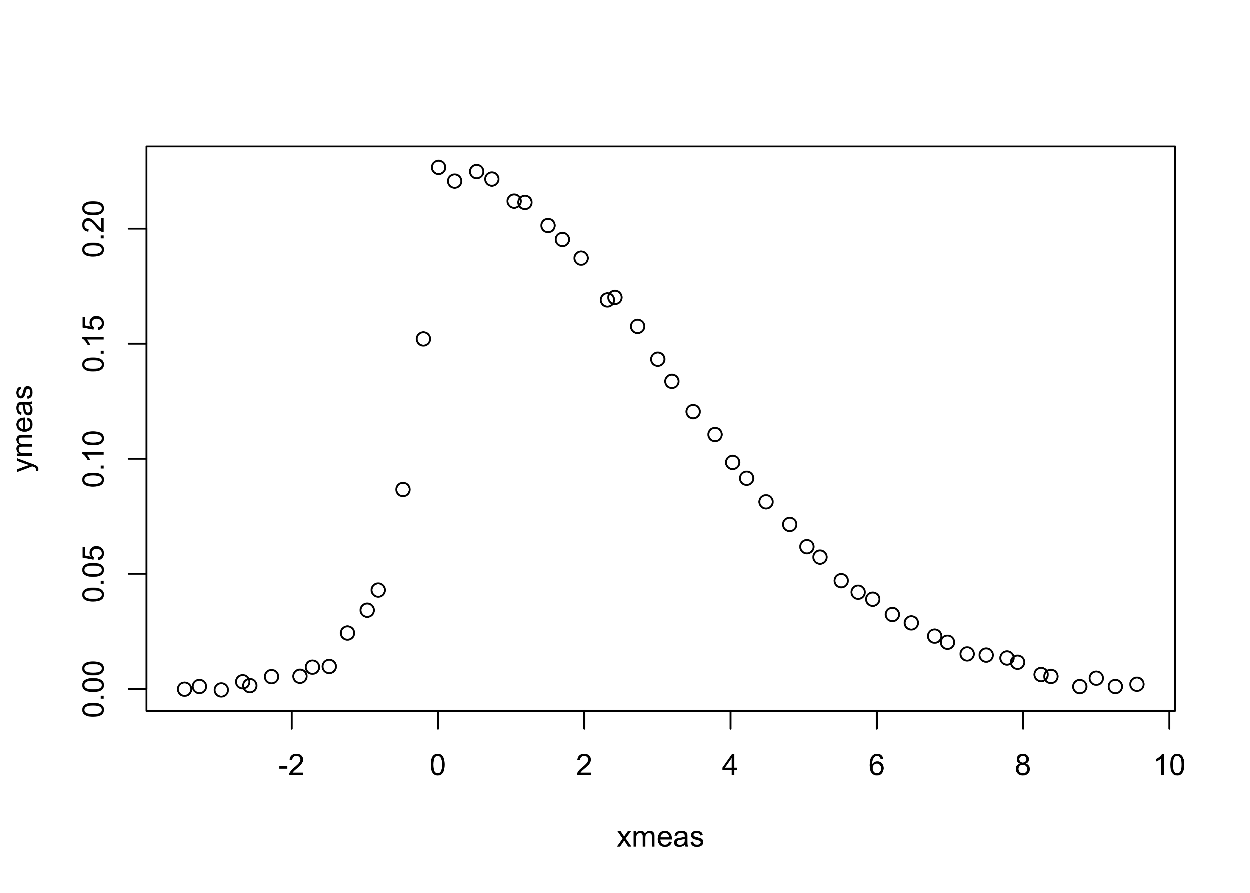
The data are contained in the file MeasData.txt which has a header line followed by lines containing \((x_{meas},y_{meas})\) pairs.
If we read in the file we can use a built-in R function, approxfun(), to create a function that approximates the data, and then use that in our computations as above:
df = read.table("MeasData.txt",header=TRUE)
xm = df$xmeas
ym = df$ymeas
rho2 = approxfun(xm,ym)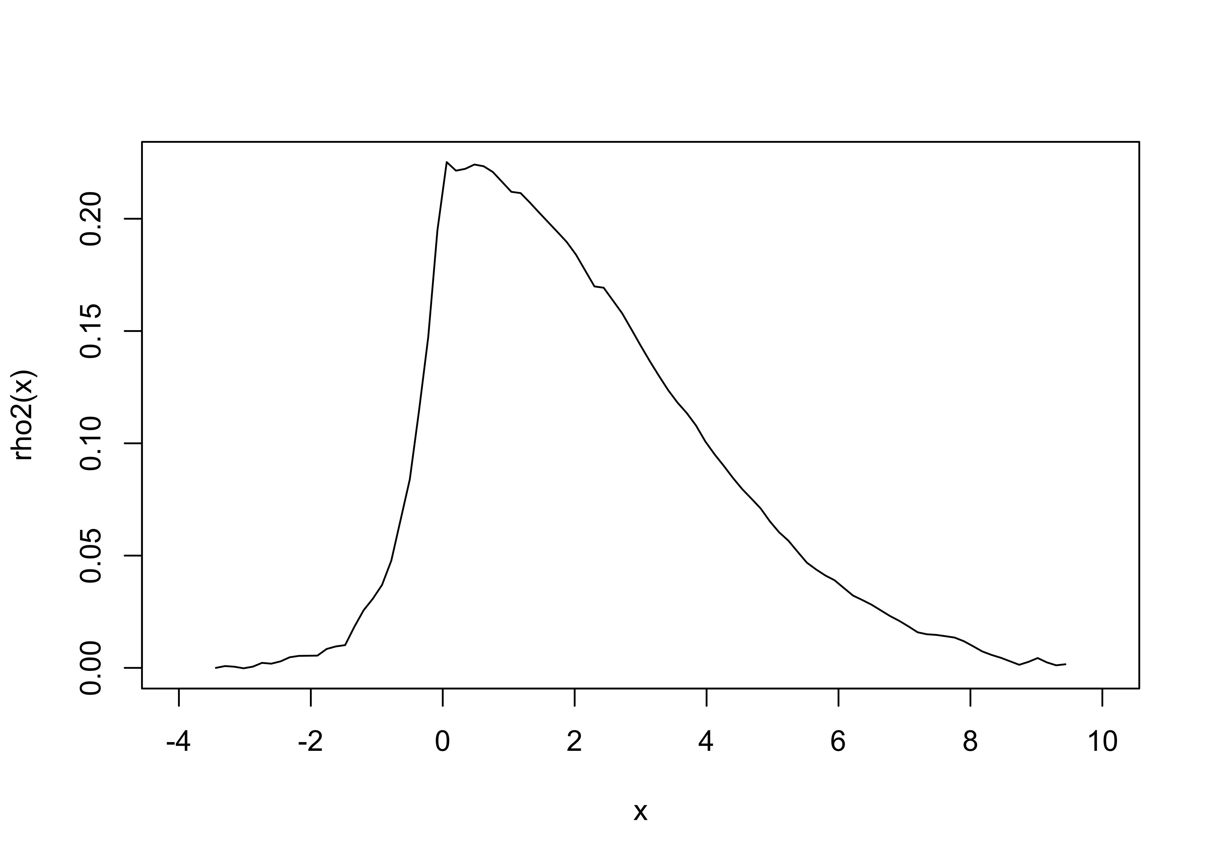
We now have our “\(\rho\)” function as before, and we can use the same process to generate a distribution of \(x\) values that mimics our measurement distribution. Rather than integrating a function, we can use approxfun() to create our \(\text{cdf}\) function from summing up our ym values.
cdf0 = cumsum(ym)/max(cumsum(ym))
cdf  = approxfun(xm,cdf0)
cdfInv = function(y){
   opInv  = function(x){abs(cdf(x)-y)}
   xout = optimize(opInv,c(-4,10))
   as.numeric(xout$minimum)
}
dtst = runif(Np,0,1)
dti = c(1:Np)*0                  # vector of initial dt of the particles
i = 0
while(i<Np){
   i = i+1
   dti[i] = cdfInv(dtst[i])
}